Overview of Error, Loss, and Cost Functions

Difference between Error, Loss, and Cost Function

In summary, the error function measures the overall performance of the model, the loss function measures the performance of the model on a single training example, and the cost function calculates the average performance of the model over the entire training set.

The error function measures the overall performance of a model on a given dataset. It is a function that takes the predicted output of a model and the actual output (or target output) and returns a scalar value that represents how well the model has performed. The error function is often used in the context of training a model, where the goal is to minimize the error function as much as possible.

The loss function, on the other hand, measures how well the model is doing on a single training example. It is a function that takes the predicted output and the actual output for a single training example and returns a scalar value representing how well the model has expected that example. The loss function is typically used to optimize the parameters of the model during training.

The cost function is the average of the loss function over the entire training set. It is a function that takes the predicted output and the actual output for each training example in the dataset and returns the average of the loss function values over all training examples. The cost function is also used to optimize the parameters of the model during training.

In this article we have the following naming convention:

\text{forecast}: h(x) \text{ and actual value}: y

Cost Functions for Regression

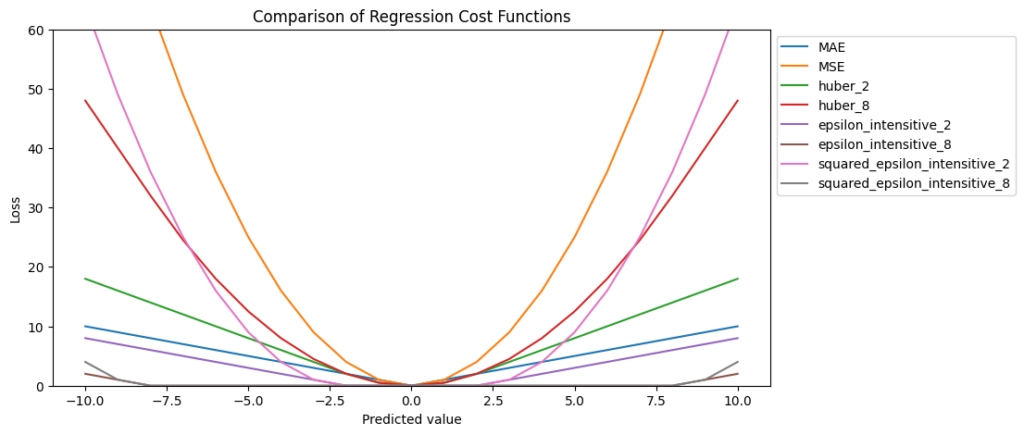
The following section describes the most used cost function for regression problems. You find the implementation and comparison of the cost functions in the google colab notebook.

Mean Absolute Error (MAE)

Mean absolute error is simply the mean of the differences between the forecast and the actual values. The MAE corresponds to the Manhattan Norm.

Mathematical Formula of MAE

MAE = {\frac{1}{n}\sum_{i=1}^{n}||h(x^{(i)})-y^{(i)}||}

Advantages of MAE

• Easy to interpret because the error is in the units of the data and forecasts.

Disadvantages of MAE

• Doesn’t penalize outliers (if needed for your model) and therefore treats all errors equally.
• Scale-dependent, therefore cannot compare to other datasets which use different units.
• For Neural Networks: The gradient of the MAE cost function will be large even for small loss values, which can lead to problems regarding convergence.

Mean Square Error (MSE)

Mean squared error is similar to MAE, but this time we square the differences between the forecasted and actual values.

Mathematical Formula of MSE

MSE= \frac{1}{n}\sum_{i=1}^{n}(h(x^{(i)})-y^{(i)})^2

Advantages of MSE

• Outliers are heavily punished (if needed for your model).
• The mean square error function is differentiable and allows for optimization using gradient descent.

Disadvantages of MSE

• The error will not be in the original units of the input data, therefore can be harder to interpret.
• Scale-dependent, therefore cannot compare to other datasets which use different units.

Root Mean Squared Error (RMSE)

The root mean squared error is the root of the mean squared error (MSE). The objective of squaring is to be more sensitive to outliers and therefore penalize large errors more. The RMSE corresponds to the Euclidian Norm.

Mathematical Formula of RMSE

RMSE= \sqrt{\frac{1}{n}\sum_{i=1}^{n}(h(x^{(i)})-y^{(i)})^2}

Advantages of RMSE

• Heavily punishes outliers (if needed for your model).
• The error is in the units of the data and forecasts.
• Kind of the best of both worlds of MSE and MAE.

Disadvantages of RMSE

• Less interpretable as you are still squaring the errors.
• Scale-dependent, therefore cannot compare to other datasets which use different units.

Huber Loss

Huber Loss combines the advantages of both Mean Absolute Error (MAE) and Mean Square Error (MSE) because Huber Loss has a linear penalty like MAE for small errors and a quadratic penalty like MSE, for large errors. This allows Huber Loss to be less sensitive to outliers compared to MSE.

Mathematical Formula of Huber

L = \begin{cases} \frac{1}{2}(h(x^{(i)})-y^{(i)})^2 & \text{for } |h(x^{(i)})-y^{(i)}| <= \delta, \\ \delta (|h(x^{(i)})-y^{(i)}| - \frac{1}{2} \delta) &  \text{otherwise} \end{cases}

From the equation, we see that Huber Loss switches from MSE to MAE past a distance of delta. After the distance of delta the error of outliers is not squared in the calculation of the loss and therefore the influence of outliers on the total error is limited.

Advantages of Huber

• The Huber Loss function is differentiable and allows for optimization using gradient descent.

Disadvantages of Huber

The choice of the delta parameter can have a significant impact on the performance of the model, and it can be challenging to select the optimal value for delta.

Epsilon Insensitive Cost Function

The Epsilon Insensitive cost function is equal to zero when the absolute difference between the true and predicted values is less than epsilon. Otherwise, the loss is equal to the absolute difference between the true and predicted values, minus epsilon. Therefore you can think about epsilon as a margin of tolerance where no penalty is given to errors.

The epsilon insensitive loss function is commonly used in support vector regression (SVR).

Mathematical Formula of Epsilon Insensitive

L = \begin{cases} 0 & \text{for } |h(x^{(i)})-y^{(i)}| <= \epsilon, \\ |h(x^{(i)})-y^{(i)}| - \epsilon &  \text{otherwise} \end{cases}

Mathematical Formula of SVM for Regression (SVR) with Epsilon Insensitive

E = \sum_{i=1}^{n}L + \frac{\lambda}{2}||w^2||

Advantages of Epsilon Insensitive Cost Function

• The Epsilon Insensitive cost function is designed to be less sensitive to outliers in the data.
• Also, the function is very flexible regarding the parameter epsilon that can be optimized to achieve the best regression solution.

Disadvantages of Epsilon Insensitive Cost Function

• While the epsilon insensitive loss function is more robust to outliers, it may sacrifice some accuracy in prediction for this robustness.
• The choice of epsilon can have a significant impact on the performance of the model. Choosing an epsilon that is too small may result in a loss function that is too sensitive to outliers, while choosing an epsilon that is too large may result in a loss function that is not sensitive enough to smaller errors.

Squared Epsilon Insensitive Cost Function

The main difference between the epsilon insensitive loss function and the squared epsilon insensitive loss function lies in how they penalize errors that exceed the threshold value, epsilon. The squared epsilon insensitive loss function penalizes errors beyond the threshold value epsilon quadratically (see also Mean Absolute Error vs. Mean Square Error).

Mathematical Formula of Epsilon Insensitive

L = \begin{cases} 0 & \text{for } |h(x^{(i)})-y^{(i)}| <= \epsilon, \\ (|h(x^{(i)})-y^{(i)}| - \epsilon)^2 &  \text{otherwise} \end{cases}

When to use Epsilon vs Squared Epsilon Insensitive Cost Function

If the data contains significant outliers, the epsilon insensitive loss function may be preferred, while the squared epsilon insensitive loss function may be more suitable for data sets with smaller amounts of noise or outliers.

Advantages of Epsilon Insensitive Cost Function

• The Squared Epsilon Insensitive cost function is very flexible regarding the parameter epsilon that can be optimized to achieve the best regression solution.

Disadvantages of Epsilon Insensitive Cost Function

• The Squared Epsilon Insensitive loss function is more sensitive to outliers and less robust to noise than the epsilon insensitive loss function.
• The choice of epsilon can have a significant impact on the performance of the model. Choosing an epsilon that is too small may result in a loss function that is too sensitive to outliers, while choosing an epsilon that is too large may result in a loss function that is not sensitive enough to smaller errors.

Quantile Loss

The Quantile Loss function does not predict the actual outcome of a regression task but predicts the corresponding quantiles of the target distribution, which can be imagined as estimating a median regression slope. Therefore the loss function measures the deviation between the predicted quantile and the actual value.

The value of gamma ranges between 0 and 1. The larger the value, the more under-predictions are penalized compared to over-predictions. For gamma equal to 0.75, under-predictions will be penalized by a factor of 0.75, and over-predictions by a factor of 0.25. The model will then try to avoid under-predictions approximately three times as hard as over-predictions, and the 0.75 quantile will be obtained. A gamma value of 0.5 equals the median.

Mathematical Formula of Quantile Loss

L= (\gamma -1)|h(x^{(i)})-y^{(i)}| + \gamma |h(x^{(i)})-y^{(i)}|

The following google colab notebook shows an end-to-end example of the Quantile Regressor

Advantages of Quantile Loss

• Instead of predicting the actual outcome, the Quantile Loss Function can predict corresponding quantiles.

Disadvantages of Quantile Loss

• The function is not differentiable at zero, which can make it difficult to use with some optimization algorithms.

MAE vs. MSE Regarding Outliers

Let’s compare the cost functions of MAE and MSE. We know that our target value is 0. Therefore, when we predict a value of 0, our cost function is also at 0, because our predicted value and target value are the same.

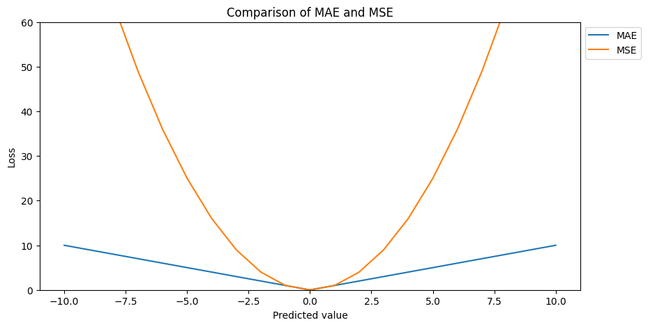
In a case, where the predictions are close to the target values the error for MAE and MSE has a small variance (values on the x-axis close to 0). For example when our predicted value on the x-axis, is around 5, then we have a loss of around 5 for the MAE cost function and around 25 for the MSE cost function.

But the further our prediction is away from our target value (in our case 0), we move away from 0 on the x-axis, the greater the difference between the error for MSE and MAE, because the MSE cost function is stepper compared to the MAE function.

This difference between the error is very important for outliers because if you have an outlier in your residuals, the MSE cost function will square the error compared to the MAE function. Finally, this will make the model with MSE loss give more weight to outliers than a model with MAE loss. The model with MSE loss will be adjusted to minimize that single outlier case at the expense of other samples, which will reduce the overall performance of the model.

Error and Loss Functions for Classification

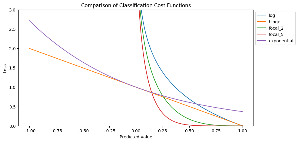
The last section of this article describes the most used cost function for classification. You find the implementation and comparison of the classification cost functions in the same google colab notebook.

Log Loss

The log loss function measures the difference between the predicted probability values and the true labels for each data point in the dataset. It applies a logarithmic transformation to the predicted probabilities to penalize incorrect predictions more severely than correct predictions. The function returns a value between 0 and infinity, with lower values indicating better model performance.

In practice, the log loss function is often used as the objective function for training classification models with gradient descent-based algorithms such as logistic regression and neural networks.

Mathematical Formula of Log Loss

L= - y^{(i)}*log(h(x^{(i)})) + (1-y^{(i)})*log(1-(h(x^{(i)}))

Log Loss and Binary Entropy Function

Log loss function and binary entropy loss function are often used interchangeably to refer to the same evaluation metric. However, strictly speaking, there is a difference between the two. The binary entropy loss function is a specific case of the log loss function that is used for binary classification problems, where there are only two possible classes.

The log loss function is a more general evaluation metric that can be used for both binary and multi-class classification problems. It extends the binary entropy loss function to handle multiple classes by using a one-vs-all approach.

Advantages of Log Loss

• Sensitive to Probabilities: The log loss function is sensitive to the predicted probabilities of the model, rather than just the predicted class labels. This makes it a more nuanced evaluation metric that can distinguish between models that make similar predictions but have different confidence levels.
• Penalizes Incorrect Predictions: The log loss function penalizes incorrect predictions more severely than correct predictions, especially for confident incorrect predictions.
• Gradient-friendly: The log loss function is differentiable and has a smooth gradient, which makes it well-suited for optimization using gradient-based algorithms such as gradient descent.
• Handle Multiclass Classification: The log loss function can be easily extended to handle multiclass classification problems using a one-vs-all approach.

Disadvantages of Log Loss

• Imbalanced Classes: The log loss function can be sensitive to class imbalance, especially in binary classification problems where one class is much rarer than the other.
• Outliers: The log loss function is sensitive to outliers, especially for confident incorrect predictions.

Hinge Loss

The hinge loss function is a commonly used loss function in machine learning for classification problems, particularly in support vector machines (SVMs). It measures the maximum margin classification error of a linear classifier and is often used for binary classification problems.
If the predicted score for the input x is on the correct side of the decision boundary, then the hinge loss is 0. If it is on the wrong side, then the hinge loss increases linearly with the distance from the decision boundary.

Mathematical Formula of Hinge Loss

L= max(0, 1- y^{(i)} * h(x^{(i)}))

Advantages of Hinge Loss

• Robust to Outliers: The hinge loss function is robust to outliers because it only penalizes misclassified examples that are close to the decision boundary.
• Suitable for Large-scale Learning: The hinge loss function can be computed efficiently and is suitable for large-scale learning problems.

Disadvantages of Hinge Loss

• Non-differentiable: The hinge loss function is non-differentiable at points where the hinge loss is 0, which can make optimization more challenging.
• Ignores Confidence: The loss function does not penalize incorrect predictions that are not confident (instance’s distance from the boundary is greater than or at the boundary). This means that a model may make many confident incorrect predictions without being penalized.
• Imbalanced Classes: The hinge loss function may not perform well for imbalanced classes, where one class is much rarer than the other.

Focal Loss

The focal loss function is a modification of the cross-entropy loss function that is commonly used for imbalanced classification problems. The function aims to address the problem of extreme class imbalance by down-weighting the contribution of easy examples and emphasizing the contribution of hard examples using the parameter gamma that controls the degree of down-weighting.

Mathematical Formula of Focal Loss

L = \begin{cases} 1-h(x^{(i)})^{\gamma} * log(h(x^{(i)})) & \text{for } y^{(i)}==1, \\ h(x^{(i)})^{\gamma} * log(1-h(x^{(i)})) &  \text{otherwise} \end{cases}

Advantages of Focal Loss

• Improved Performance on Imbalanced Datasets: The focal loss function is designed to address the problem of class imbalance in datasets by focusing on hard examples and down-weighting the contribution of easy examples.
• Can be Used with Deep Learning Models: The focal loss function can be used with a wide range of deep learning models, including convolutional neural networks (CNNs) and recurrent neural networks (RNNs).
• Flexible: The degree of down-weighting can be controlled by the gamma hyperparameter, which can be tuned to suit the specific needs of the problem.

Disadvantages of Focal Loss

• Increased Computational Complexity: The focal loss function involves additional computations compared to the standard cross-entropy loss function, which can increase the computational complexity of training the model.
• Hyperparameter Tuning: The degree of down-weighting is controlled by the gamma hyperparameter, which needs to be tuned carefully to achieve good performance.

Exponential Loss

The exponential loss function is a commonly used loss function in machine learning for binary classification problems. It is also known as the “exponential hinge loss” or “AdaBoost loss”. The exponential loss function is similar to the hinge loss function used in SVMs, but instead of being linear, it is an exponential function of the margin.

Mathematical Formula of Exponential Loss

L= exp(-y^{(i)} * h(x^{(i)}))

Advantages of Exponential Loss

• Well-Suited for Boosting Algorithms: The exponential loss function is commonly used in boosting algorithms such as AdaBoost, as it is well-suited to handle noisy or mislabeled data.
• Can Produce High-Quality Probability Estimates: The exponential loss function is known to produce high-quality probability estimates, which can be useful in certain applications such as risk assessment.

Disadvantages of Exponential Loss

• Sensitive to Outliers: The exponential loss function can be sensitive to outliers, as it assigns very high penalties to examples that are misclassified with high confidence.
• Not as Robust to Class Imbalance: The exponential loss function is not as robust to class imbalance as some other loss functions, such as the focal loss function.
• Computationally Expensive: The exponential loss function can be computationally more expensive than some other loss functions.

Read my latest articles:

• Evaluate Clustering Algorithms
• Decision Tree
• Transform the Target Variable
• Feature Transformation in Machine Learning
• Overview of Error, Loss, and Cost Functions