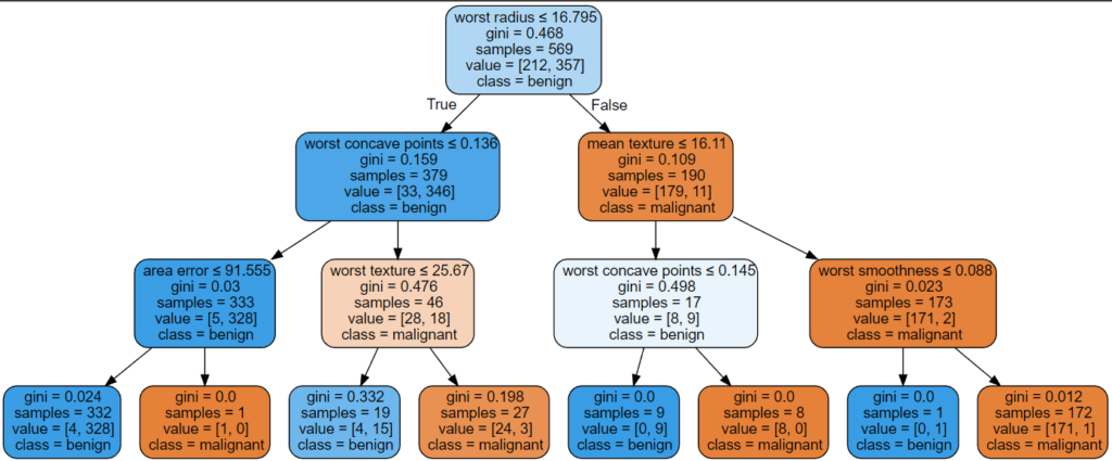
Decision Tree

During the training of the decision tree algorithm for a classification task, the dataset is split into subsets on the basis of features.

• If one subset is pure regarding the labels of the dataset, splitting this branch is stopped.
• If the subset is not pure, the splitting is continued.

After the training, the overall importance of a feature in a decision tree can be computed in the following way:
1) Go through all the splits for which the feature was used and measure how much it has reduced the impurity compared to the parent node.
2) The sum of all importance is scaled to 100. This means that each importance can be interpreted as a share of the overall model importance.

You can also plot the finished decision tree in your notebook.

If you do not know how, no problem, I created two end-to-end examples with Google Colab.

Definitions of Decision Trees

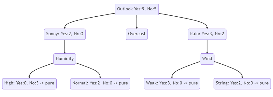
Before we look at the decision tree in more detail, we need to get to know its individual elements of it. There are already names of the nodes from the following example listed.

• Root Node: represents the whole sample and gets divided into sub-trees.
• Splitting: the process of dividing a node into two or more sub-nodes.
• Decision Node: node, where a sub-node splits into further sub-nodes → Wind
• Leaf: nodes that can not split anymore are called terminal nodes (pure) → Overcast
• Sub-Tree: sub-section of the entire tree
• Parent and Child Node: A node, which is divided into sub-nodes is called the parent node of sub-nodes where as sub-nodes are the child of the parent’s node. → Weak and Strong are child nodes of parent Wind.

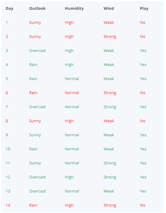
The following table shows a dataset with 14 samples, 3 features, and the label “Play” that we will use as an example to train a decision tree classifier by hand.

The following decision tree shows what the final decision tree looks like. The tree has a depth of 2 and at the end all nodes are pure. You see that in the first step, the dataset is divided by the feature “Outlook”. In the second step the previous divided feature “Sunny” is divided by “Humidity” and “Rain” is divided by “Wind”.

You might ask yourself how we know which feature we should use to divide the dataset. We will answer this question in the last section of this article.

Decision Tree Advantages & Disadvantages

Decision Tree Advantages

• The main advantage of decision trees is, that they can be visualized and therefore are simple to understand and interpret.
  • Therefore visualize the decision tree as you are training by using the export function (see the Google Colab examples). Use max_depth=3 as an initial depth, because the tree is easy to visualize and overview. The objective is to get a feeling for how well the tree is fitting your data.
• Requires little data preparation, because decision trees do not need feature scaling, encoding of categorical values, or imputation of missing values. However, if you are using sklearn, you have to input all missing values, because the current implementation does not support missing values. Also if you want that the decision tree works with categorical values, you have to use the sklearn implementation of HistGradientBoostingRegressor and HistGradientBoostingClassifier.
• Decision tree predictions are very fast on large datasets, because the cost of using the tree (predicting data) is logarithmic in the number of data points used to train the tree. Note that only the prediction is very fast, not the training of a decision tree.
• Decision trees are able to handle multi-output classification problems.

Decision Tree Disadvantages

• Decision Trees have a tendency to overfit the data and create an over-complex solution that does not generalize well.
  • How to avoid overfitting is described in detail in the “Avoid Overfitting of the Decision Tree” section
• Decision trees can be unstable because small variations in the data might result in a completely different tree being generated.
  • Use ensemble techniques, either stacking with other machine learning algorithms or bagging techniques like Random Forst to avoid this problem.
• There are concepts that are hard to learn for decision trees because trees do not express them easily, such as XOR, parity, or multiplexer problems.
• If your dataset is unbalanced, decision trees will likely create biased trees.
  • You can balance your dataset before training by balancing techniques like SMOTE or preferably by normalizing the sum of the sample weights sample_weights for each class to the same value.
  • If the samples are weighted, it will be easier to optimize the tree structure using the weight-based pre-pruning criterion min_weight_fraction_leaf, which ensures that leaf nodes contain at least a fraction of the overall sum of sample weights.

Avoid Overfitting of the Decision Tree

Before Training the Decision Tree

We know that decision trees tend to overfit data with a large number of features. Getting the right ratio of samples to the number of features is important since a tree with few samples in high dimensional space is very likely to overfit. Therefore we can use different dimensionality reduction techniques beforehand to limit the number of features the decision tree is able to be trained on.

During Training the Decision Tree

To avoid overfitting the training data, we need to restrict the size of the Decision Tree during training. The following chapter shows the parameter overview and how to prevent overfitting during the training.

After Training the Decision Tree

After training the decision tree, we can prune the tree. The following steps are done when pruning is performed.

1. Train the decision tree to a large depth
2. Start at the bottom and remove leaves that are given negative returns when compared to the top.

You can use the Minimal Cost-Complexity Pruning technique in sklearn with the parameter ccp_alpha to perform pruning of regression and classification trees.

Decision Tree Parameter Overview

The following list gives you an overview of the main parameters of the decision tree, how to use these parameters, and how you can use the parameter against overfitting.

• criterion: The function that is used to measure the quality of a split
  • Classification: can be Gini, Entropy, or Log Loss
  • Regression: can be Squared Error, Friedman MSE, Absolute Error, or Poisson
• max_depth: The maximum depth of the tree
  • Initial search space: int 2…4
  • The number of samples required to populate the tree doubles for each additional level the tree grows to.
  • Overfitting: when the algorithm is overfitting, reduce max_depth, because a higher depth will allow the model to learn relations very specific to a particular sample.
• min_samples_split: The minimum number of samples required to split an internal node
  • Initial search space: float 0.1…0.4
  • Overfitting: when the algorithm is overfitting, increase min_samples_split, because higher values prevent a model from learning relations that might be highly specific to the particular sample selected for a tree.
• min_samples_leaf: The minimum number of samples required to be at a leaf node. A split point at any depth will only be considered if it leaves at least min_samples_leaf training samples in each of the left and right branches.
  • Initial search space: float 0.1…0.4
  • Generally, lower values should be chosen for imbalanced class problems because the regions in which the minority class will be in majority will be very small.
  • For classification with few classes, min_samples_leaf=1 is often the best choice.
  • Overfitting: when the algorithm is overfitting, increase min_samples_leaf
• max_leaf_nodes: The maximum number of terminal nodes or leaves in a tree.
  • Can be defined in place of max_depth. Since binary trees are created, a depth of n would produce a maximum of 2^n leaves.
• max_features: The number of features to consider while searching for the best split.
  • The features will be randomly selected.
  • As a thumb-rule, the square root of the total number of features works great but we should check up to 30-40$% of the total number of features.
  • Overfitting: Higher values can lead to overfitting.
• min_impurity_decrease: If the weighted impurity decrease is greater than the min_impurity_decrease threshold, the node is split.
  • Overfitting: when the algorithm is overfitting, increase min_impurity_decrease

The following Google Colab shows the differences of different parameters on the trained decision tree as well as the performance of the model for a classification task.

How to use Decision Trees for Regression

In most cases, decision trees are used for classification, but it is also possible to use decision trees for regression. The main difference is that instead of predicting a class in each node, it predicts a value. You can find an end-to-end example of how to use decision trees for regression in the following Google Colab. Also, all charts from this section are in the notebook.

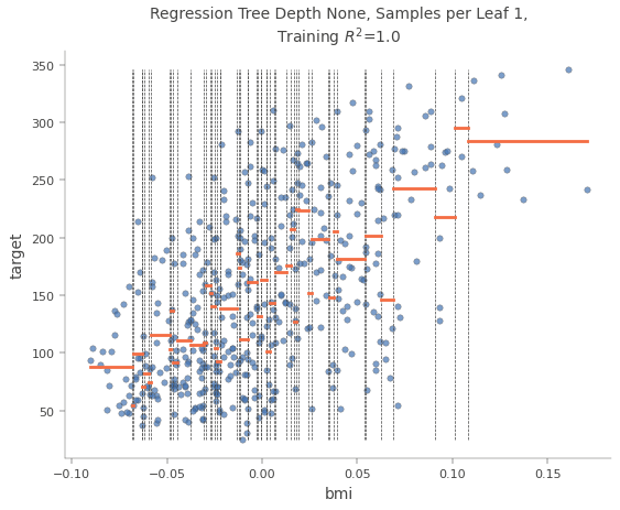
The following picture shows how the dataset was divided by the feature “bmi”. The value of the target variable is the median of all values in the sub-nodes.

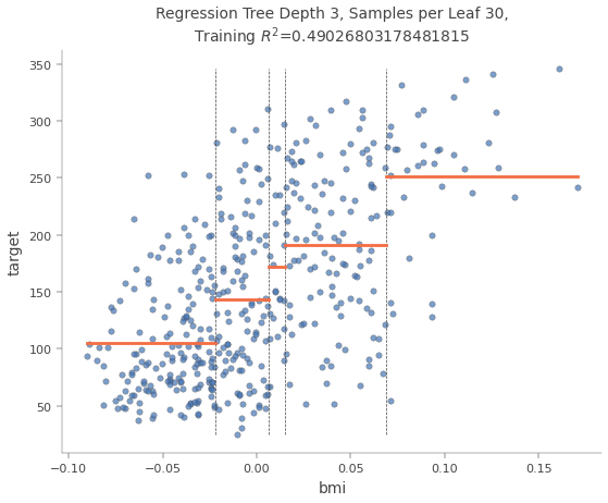
You see that when the prediction would only be done by this one feature “bmi” there would be only 5 different values for the output. With a deeper decision tree, you have more values for the output but you see the general problem with decision trees in regression tasks. Therefore if you have a regression task my suggestion is not to use decision trees in the first place, but to focus on other machine learning algorithms, because they likely will have a better performance.

Just like for classification tasks, Decision Trees are prone to overfitting when dealing with regression tasks. Without any regularization (i.e., using the default hyperparameters), you get the predictions in the following chart, which is trained on the same dataset as the decision tree from the previous decision tree. The only difference is that the decision tree that is overfitting was trained with standard parameters and the decision tree from the previous scatter-plot was limited to max_depth=3 and min_samples_leaf=30.

How to Select the Feature for Splitting?

The decision of which features are used for splitting heavily affects the accuracy of the model. Decision trees use multiple algorithms to decide to split a node into two or more sub-nodes. The creation of sub-nodes increases the homogeneity of the resulting sub-nodes. The decision tree splits the nodes on all available variables and then selects the split which results in the most homogeneous sub-nodes and therefore reduces the impurity. The decision criteria are different for classification and regression trees. The following are the most used algorithms for splitting decision trees:

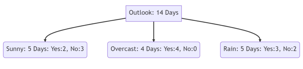
Split on Outlook

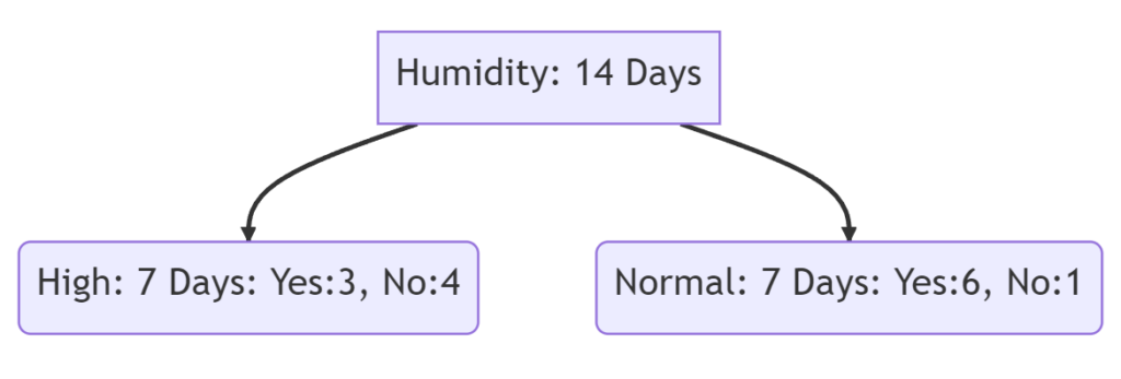
Split on Humidity

Gini Index

The Gini coefficient is a measure of statistical dispersion and is the most commonly used measure of inequality. The Gini coefficient measures the inequality among values of a frequency distribution. A Gini coefficient of zero expresses perfect equality, where all values are the same, whereas a Gini coefficient of 1 (100%) expresses maximal inequality among values.

The following lines show the calculation of the Gini index when we split for “Outlook” and “Humidity” in the first decision node.

Split on Outlook

G(sunny) = (\frac{2}{5})^2 + (\frac{3}{5})^2 = 0.52 \\
G(overcast) = (\frac{4}{4})^2 + (\frac{0}{4})^2 = 1 \\
G(rain) = (\frac{3}{5})^2 + (\frac{2}{5})^2 = 0.52 \\

G(Outlook) = \frac{5*0.52 + 4*1 + 5*0.52}{14} = 0.657

Split on Humidity

G(high) = (\frac{3}{7})^2 + (\frac{4}{7})^2 = 0.51 \\
G(normal) = (\frac{6}{7})^2 + (\frac{1}{7})^2 = 0.75

G(Humidity) = \frac{7*0.51 + 7*0.75}{14} = 0.63

We see that the Fini coefficient for “Outlook” with 0.657 is higher compared to “Humidity” with 0.63. Therefore when we would use the Gini Index as a criterion to divide the dataset, the first node would be split the dataset by “Outlook”.

Entropy

Entropy is the expected value (mean) of the information of an event. The objective of entropy is to define information as a negative of the logarithm of the probability distribution of possible events or messages. As a result of the Shannon entropy, the decision tree algorithm tries to reduce the entropy with every split as much as possible. Therefore the feature for splitting is selected which reduces the entropy most until an entropy of 0 is achieved and the category of the feature is pure.

E(parent node) = -(\frac{9}{14})*\log_2(\frac{9}{14})-(\frac{5}{14})*\log_2(\frac{5}{14})=0.94

Split on Outlook

E(sunny) = -(\frac{2}{5})*\log_2(\frac{2}{5})-(\frac{3}{5})*\log_2(\frac{3}{5})=0.97 \\
E(overcast) = -(\frac{4}{4})*\log_2(\frac{4}{4})-(\frac{0}{4})*\log_2(\frac{0}{4})=0 \\
E(rain) = -(\frac{3}{5})*\log_2(\frac{3}{5})-(\frac{2}{5})*\log_2(\frac{2}{5})=0.97

E(Outlook) = \frac{5}{14}*0.97+\frac{4}{14}*0+\frac{5}{14}*0.97=0.69

Split on Humidity

E(high) = -(\frac{3}{7})*\log_2(\frac{3}{7})-(\frac{4}{7})*\log_2(\frac{4}{7})=0.99 \\
E(normal) = -(\frac{6}{7})*\log_2(\frac{6}{7})-(\frac{1}{7})*\log_2(\frac{1}{7})=0.59

E(Humidity) = \frac{7}{14}*0.99+\frac{7}{14}*0.59=0.79

From the example, you see that we would divide the dataset by “Outlook” again because the entropy is reduced the most to 0.69 from 0.94.

Variance

Reduction in variance is an algorithm used for continuous target variables (regression problems). This algorithm uses the standard formula of variance to choose the best split. The split with lower variance is selected as the criteria to split the samples. Assumption: numerical value 1 for playing and 0 for not playing.

\text{parent node mean} = \frac{9*1+5*0}{14} = 0.64 \Rightarrow
V(\text{parent node}) = \frac{9(1-0.64)^2+5(0-0.64)^2}{14} = 0.97

Split on Outlook

\text{sunny mean} = \frac{2*1+3*0}{5} = 0.4 \Rightarrow
V(\text{sunny}) = \frac{2(1-0.4)^2+3(0-0.4)^2}{5} = 0.24 \\

\text{overcast mean} = \frac{4*1+0*0}{4} = 1 \Rightarrow
V(\text{overcast}) = \frac{4(1-1)^2+0(0-1)^2}{4} = 0 \\

\text{rain mean} = \frac{3*1+2*0}{5} = 0.6 \Rightarrow
V(\text{rain}) = \frac{3(1-0.6)^2+2(0-0.6)^2}{5} = 0.24

V(outlook) = \frac{5}{14}*0.24 + \frac{4}{14}*0 + \frac{5}{14}*0.24 = 0.17

Split on Humidity

\text{high mean} = \frac{3*1+4*0}{7} = 0.43 \Rightarrow
V(\text{high}) = \frac{3(1-0.43)^2+4(0-0.43)^2}{7} = 0.24 \\

\text{normal mean} = \frac{6*1+1*0}{7} = 0.86 \Rightarrow
V(\text{high}) = \frac{6(1-0.86)^2+1(0-0.86)^2}{7} = 0.12

V(humidity) = \frac{7}{14}*0.24 + \frac{7}{14}*0.12 = 0.18

Because the variance of “Outlook” is lower compared to “Humidity” (0.17 vs. 0.18), the dataset would be divided by “Outlook”.

Read my latest articles:

• Evaluate Clustering Algorithms
• Decision Tree
• Transform the Target Variable
• Feature Transformation in Machine Learning
• Overview of Error, Loss, and Cost Functions