Evaluate Clustering Algorithms

The difference in Performance Measurement between Supervised and Unsupervised Learning

The performance measurement for supervised learning algorithms is simple because the evaluation can be done by comparing the prediction against the labels. However, for an unsupervised learning problem, there are no labels and therefore also no ground truth. Therefore we need other evaluation methods to determine how well our clustering algorithm performs. First, let’s start to find out what a good clustering algorithm is.

A good clustering algorithm has two characteristics
1) A clustering algorithm has a small within-cluster variance. Therefore all data points in a cluster are similar to each other.
2) Also a good clustering algorithm has a large between-cluster variance and therefore clusters are dissimilar to other clusters.

All clustering performance measurements are based on these two characteristics. Generally, there are two types of evaluation metrics for clustering,

• Extrinsic Measures: These measures require ground truth labels, which may not be available in practice
  • Rand Index
  • Mutual Information
  • V-Measure
  • Fowlkes-Mallows Score
• Intrinsic Measures: These measures do not require ground truth labels (applicable to all unsupervised learning results)
  • Silhouette Coefficient

In the following chapters, we dive into these cluster performance measurements.

Rand Index

\text{Rand Index} = \frac{\text{Number of pair-wise same cluster} + \text{Number of pair-wise wrong cluster}}{\text{Total number of possible pairs}}

where the total number of possible pairs is calculated by

\text{Total number of possible pairs} = \frac{n*(n-1)}{2}

where n is the number of samples in the dataset.

Adjusted Rand Index (ARI)

Because there might be many cases of “true negative” pairs by randomness, the Adjusted Rand Index (ARI) adjusts the RI by discounting a chance normalization term.

When to use the Rand Index?

• If you prefer interpretability: The Rand Index offers a straightforward and accessible measure of performance.
• If you have doubts about the clusters: The Rand Index and Adjusted Rand Index do not impose any preconceived notions on the cluster structure, and can be used with any clustering technique.
• When you need a reference point: The Rand Index has a value range between 0 and 1, and the Adjusted Rand Index range between -1 and 1. Both defined value ranges provide an ideal benchmark for evaluating the results of different clustering algorithms.

When not to use the Rand Index?

• Do not use the Rand Index if you do not have the ground truth labels: RI and ARI are extrinsic measures and require ground truth cluster assignments.

Example of How to Calculate the Rand Index

The following picture shows an example of how the Rand Index is calculated. We have a dataset that consists of 6 samples (A-F) and two cluster algorithms that made their prediction for each sample if the sample belongs to clusters 1, 2, or 3 (see the first table in the picture). In the second table, all possible sample pairs are listed with the predicted cluster for algorithms 1 and 2.

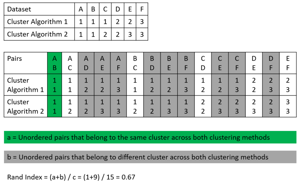
To calculate the Rand Index we search for

• Number of the pair-wise same cluster (unordered pairs that belong to the same cluster across both clustering methods), seen in green
• Number of the pair-wise wrong clusters (unordered pairs that belong to different clusters across both clustering methods), seen in gray

Based on the values we found in this example, we can compute the Rand Index:

\text{Rand Index} = \frac{\text{Number of pair-wise same cluster} + \text{Number of pair-wise wrong cluster}}{\text{Total number of possible pairs}} = \frac{1 + 9}{15} = 0.67

Calculate the Rand Index in Python

I also proved my example with a short implementation in Python with Google Colab. You see that the Rand Index is equal in the Python implementation as well as in the manual calculation.

from sklearn.metrics import rand_score, adjusted_rand_score

labels = [1, 1, 1, 2, 2, 3]  
labels_pred = [1, 1, 2, 2, 3, 3]
  
RI = rand_score(labels, labels_pred)
# Rand Index: 0.6666666666666666

ARI = adjusted_rand_score(labels, labels_pred)

Mutual Information

\text{Mutal Information (MI)} = \sum_{i=1}^{|U|} \sum_{j=1}^{|V|} P(i,j) log \frac{P(i,j)}{P(i)P'(j)}

\text{Normalized Mutal Information (NMI)} = \frac{MI}{\frac{1}{2}[H(U)+H(V)]}

\text{Adjusted Mutal Information (AMI)} = \frac{MI-E[MI]}{\frac{1}{2}[H(U)+H(V)]-E[MI]}

where

• U: class labels
• V: cluster labels
• H: Entropy

When to use Mutual Information?

• You need a reference point for your analysis: MI, NMI, and AMI are bounded between the [0, 1] range. The bounded range makes it easy to compare the scores between different algorithms.

When not to use Mutual Information?

• Do not use the Mutual Information measurement if you do not have the ground truth labels: MI, NMI, and AMI are extrinsic measures and require ground truth cluster assignments.

Example of how to calculate Mutual Information

Assume we have m=3 classes and k=2 clusters that you see in the following picture.

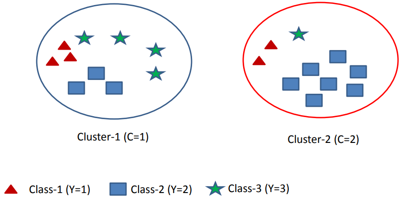
Calculate the Entropy of Class Labels

The Entropy of Class Labels is calculated for the entire dataset and therefore independent of the clustering output. Therefore you can calculate the Entropy of Class Labels prior to clustering.

P(Y=1)=\frac{5}{20}=0.25

P(Y=2)=\frac{5}{20}=0.25

P(Y=3)=\frac{10}{20}=0.5

H(Y)=-0.25 \log(0.25) -0.25 \log(0.25) -0.5 \log(0.5) = 1.5

Calculate the Entropy of Cluster Labels

The Entropy of Cluster Labels changes every time the clustering changes.

P(C=1)=\frac{10}{20}=0.5

P(C=2)=\frac{10}{20}=0.5

H(C)=-0.5 \log(0.5) -0.5 \log(0.5) = 1

Calculate the Entropy of Class Labels within each Cluster

Entropy of Class Labels in Cluster 1

P(Y=1|C=1) = \frac{3}{10}

P(Y=2|C=1) = \frac{3}{10}

P(Y=2|C=1) = \frac{4}{10}

H(Y|C=1) = -P(C=1) \sum_{y \in \{1,2,3 \}} P(Y=y|C=1) log(P(Y=y|C=1)) \\ = -0.5*[\frac{3}{10}log(\frac{3}{10}) + \frac{3}{10}log(\frac{3}{10}) + \frac{4}{10}log(\frac{4}{10})] = 0.7855

Entropy of Class Labels in Cluster 2

P(Y=1|C=2) = \frac{2}{10}

P(Y=2|C=2) = \frac{7}{10}

P(Y=2|C=2) = \frac{1}{10}

H(Y|C=2) = -P(C=2) \sum_{y \in \{1,2,3 \}} P(Y=y|C=2) log(P(Y=y|C=2)) \\ = -0.5*[\frac{2}{10}log(\frac{2}{10}) + \frac{7}{10}log(\frac{7}{10}) + \frac{1}{10}log(\frac{1}{10})] = 0.5784

Calculate the Mutual Information

MI = H(Y) - H(Y|C) = 1.5-[0.7855+0.5784] = 0.1361

NMI = \frac{MI}{\frac{1}{2}[H(U)+H(V)]} = \frac{2*0.1361}{1.5+1} = 0.1089

Calculate Mutual Information in Python

from sklearn.metrics import (mutual_info_score, normalized_mutual_info_score, adjusted_mutual_info_score)

labels = [0, 0, 0, 1, 1, 1]  
labels_pred = [1, 1, 2, 2, 3, 3]  
  
MI = mutual_info_score(labels, labels_pred)  
NMI = normalized_mutual_info_score(labels, labels_pred)  
AMI = adjusted_mutual_info_score(labels, labels_pred)

V-Measure

Components of the V-Measure

Homogeneity (h)

Homogeneity measures how much the sample in a cluster are similar. It is defined using Shannon’s entropy.

h = 1-\frac{H(C|K)}{H(C)}

where H: Entropy

H(C|K) = -\sum_{c,k}\frac{n_{ck}}{N} * log(\frac{n_{ck}}{n_k})

If we look at the term H(C|K) it contains n_ck/n_k which represents the ratio between the number of samples labeled c in cluster k and the total number of samples in cluster k. Therefore, if all samples in cluster k have the same label c, the homogeneity equals 1, see the following picture for visualization.

Completeness (c)

Completeness although measures how much similar samples are put together by the clustering algorithm.

c = 1-\frac{H(K|C)}{H(K)}

where H is also the entropy that contains the term n_ck/n_c which represents the ratio between the number of samples labeled c in cluster k and the total number of samples labeled c. When all samples of kind c have been assigned to the same cluster k, the completeness equals 1.

When to use V-measure?

• You want interpretability: V-measure provides a clear understanding of cluster quality through its homogeneity and completeness metrics.
• You are uncertain about cluster structure: V-measure is a flexible measure that can be used with any clustering algorithm, regardless of the underlying structure.
• You want a basis for comparison: The bounded range of V-measure, homogeneity, and completeness between 0 and 1 is useful for comparing the effectiveness of different clustering algorithms.

When not to use V-measure?

• If you lack true labels: V-measure, homogeneity, and completeness are extrinsic measures that require ground truth labels to assess cluster quality accurately.
• If your dataset is small (<1000 samples) and has many clusters (>10): The v-measure does not adjust for chance and may yield non-zero scores even with random labeling, especially with many groups.

Calculate the V-measure in Python

from sklearn.metrics import homogeneity_score, completeness_score, v_measure_score

labels = [0, 0, 0, 1, 1, 1]  
labels_pred = [1, 1, 2, 2, 3, 3]  
  
HS = homogeneity_score(labels, labels_pred)  
CS = completeness_score(labels, labels_pred)  
V = v_measure_score(labels, labels_pred, beta=1.0)

Silhouette Coefficient

\text{Silhouette Score} = \frac{b-a}{max(a,b)}

where

• a: average intra-cluster distance (the average distance between each point within a cluster)
• b: average inter-cluster distance (the average distance between all clusters)

Average intra-cluster distance

For every data point i in C_I (data point i in the cluster C_I) let

a(i) = \frac{1}{|C_I|-1} \sum_{j \in C_I, i \neq j} d(i,j)

be the distance between i and all other data points in the same cluster, where

• |C_I| is the number of points belonging to cluster i and
• d(i,j) is the distance between data points i and j in cluster C_I

Average inter-cluster distance

For every data point i in C_I (data point i in the cluster C_I) let

b(i) = min_{J \neq I}\frac{1}{|C_J|} \sum_{j \in C_J} d(i,j)

to be the smallest (therefore the min operator) mean distance of i to all points in any other cluster (any cluster of which i is not a member), where

• |C_J| is the number of points belonging to cluster J and
• d(i,j) is the distance between data points i and j in cluster C_J

Interpretation of the Silhouette Coefficient

• SC near +1: indicates that the sample is far away from the neighboring clusters
• SC of 0: indicates that the sample is on or very close to the decision boundary between two neighboring clusters
• SC near -1: indicates that those samples might have been assigned to the wrong cluster

Visualizing the Silhouette Coefficient via Silhouette Plots

The following example shows the silhouette plots of clustering with a different number of clusters. Based on the silhouette plots, we can choose the optimal number of clusters.

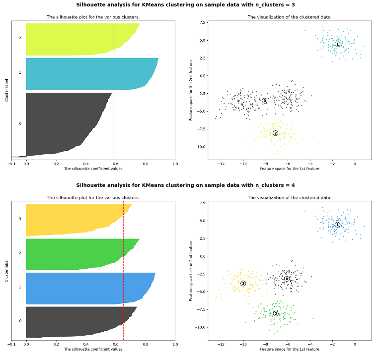
The silhouette plots show the following results:

• We would prefer a number of clusters of 4 instead of 3, because due to the presence of groups with below-average silhouette scores (see cluster 0 for n_clusters=3, the black shape does not reach the red dotted line that represents the average silhouette scores) and also due to wide fluctuations in the size of the silhouette plots.
• The thickness of the silhouette plot shows the cluster size. The silhouette plot for cluster 0 when n_clusters=3, is more significant in size owing to the grouping of the 2 sub-clusters (clusters 0 & 3 for n_clusters=4) into one big group.

When to use the Silhouette Coefficient?

• The Silhouette Coefficient is intuitive and easy to understand because you can use the Silhouette plots to visualize the results. Therefore the Silhouette Coefficient has a high interpretability
• Silhouette Coefficient has a value range of [-1, 1], from incorrect to highly dense clustering, with 0 overlapping clusters. The bounded range makes it easy to compare the scores between different algorithms.
• If you value well-defined clusters: The Silhouette Coefficient aligns with the common notion of good clusters, which are both dense and well-separated.

When not to use the Silhouette Coefficient?

If you are evaluating various clustering approaches: The Silhouette Coefficient may give an advantage to density-based clustering methods, and thus, may not be an equitable comparison metric for other types of clustering algorithms.

Calculate Silhouette Coefficient in Python

from sklearn.metrics import silhouette_score

data = [  
	[5.1, 3.5, 1.4, 0.2],  
	[4.9, 3. , 1.4, 0.2],  
	[4.7, 3.2, 1.3, 0.2],  
	[4.6, 3.1, 1.5, 0.2],  
	[5. , 3.6, 1.4, 0.2],  
	[5.4, 3.9, 1.7, 0.4],  
	]

clusters = [1, 1, 2, 2, 3, 3]
  
s = silhouette_score(data, clusters, metric="euclidean")

Fowlkes-Mallows Score

\text{FM} = \sqrt{\frac{TP}{TP+FP} * \frac{TP}{TP+FN}}

where

• TP: the number of pairs of points that belong to the same clusters in both the true labels and the predicted labels.
• FP: the number of pairs of points that belong to the same clusters in the true labels and not in the predicted labels.
• FN: the number of pairs of points that belongs in the same clusters in the predicted labels and not in the true labels.

When to use the Fowlkes-Mallows Score?

• If you have doubts about the clusters: The Fowlkes-Mallows Score is a versatile measure that does not impose any assumptions on the underlying cluster structure, making it suitable for all clustering techniques.
• You want a basis for comparison: The bounded range of the Fowlkes-Mallows Score between 0 and 1 offers a convenient benchmark for evaluating the performance of different clustering algorithms.

When not to use the Fowlkes-Mallows Score?

• You do not have the ground truth labels: Fowlkes-Mallows Scores are extrinsic measures and require ground truth cluster assignments.

Example of How to Calculate the Fowlkes-Mallows Score

The following picture shows how to calculate the Fowlkes-Mallows Score.

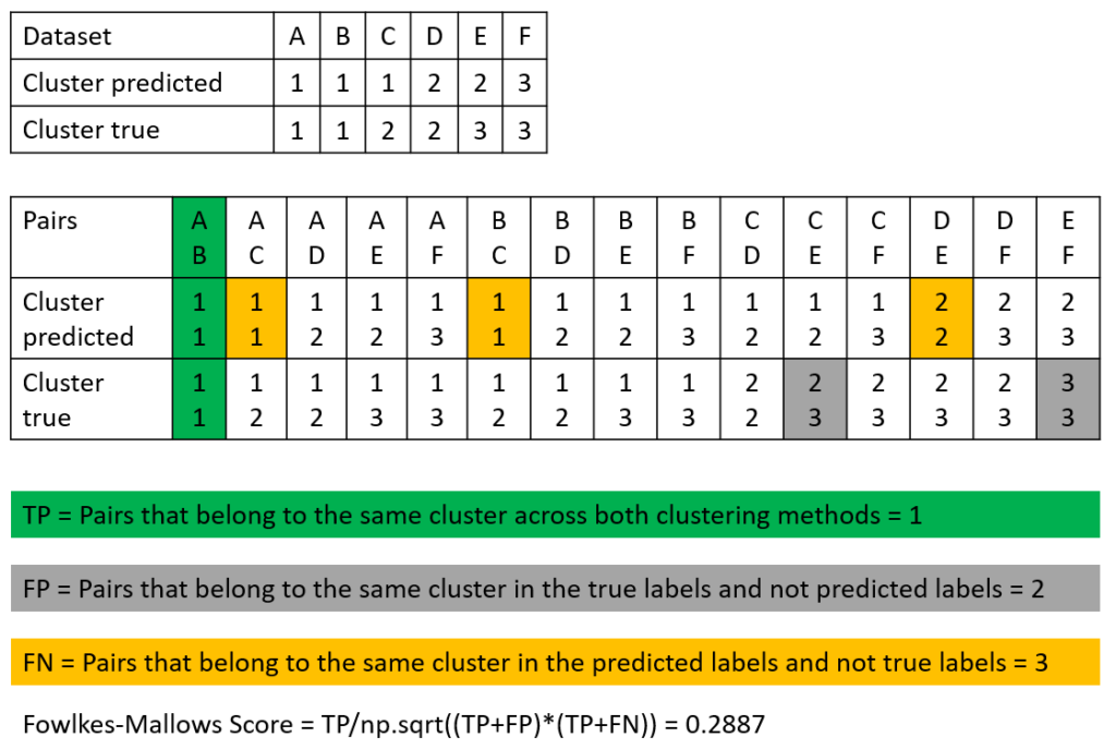
Like in the example where we calculated the Rand Index, we analyze all value pairs from the dataset and their predicted clusters. Note that we only count the value pairs, so all TP pairs, as well as FP and FN are counted per value pair, even if for the TP values, the value pair is the same in the predicted and true cluster (we do not count by the number of clusters).

In the following section, I also computed the same example in Python to prove that the results from the example are correct.

Calculate the Fowlkes-Mallows Score in Python

The following Google Colab shows the implementation of all the clustering performance measurements in this article. The last implementation is the computation of the Fowlkes-Mallows Score from our example.

from sklearn.metrics import fowlkes_mallows_score

labels = [0, 0, 0, 1, 1, 1]
labels_pred = [1, 1, 2, 2, 3, 3]

FMI = fowlkes_mallows_score(labels, labels_pred)

Read my latest articles:

• Evaluate Clustering Algorithms
• Decision Tree
• Transform the Target Variable
• Feature Transformation in Machine Learning
• Overview of Error, Loss, and Cost Functions