In machine learning, feature transformation is a common technique used to improve the accuracy of models. One of the reasons for transformation is to handle skewed data, which can negatively affect the performance of many machine learning algorithms.
In this article, you
- learn how to decide if you should apply a transformer to your feature and
- get to know different transformers with their advantages and disadvantages.
Table of Contents
Programming Example for Feature Transformation
For this article, I programmed an example to work with. First I created a positively skewed distribution and applied different transformations with the objective to make the transformed distribution more normal. The following bar plot shows the results of the transformation.
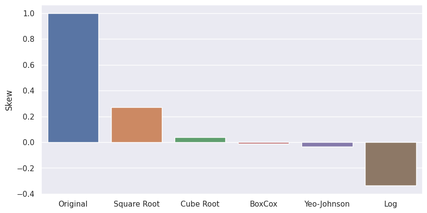
- The square root distribution reduces the skewness and maintains the positive skewness.
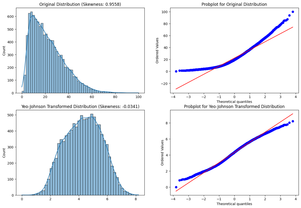
- The Cube Root and Yeo-Johnson transformer work very well on the dataset.
- The Box-Cox transformation reduces the skewness to almost 0 and is therefore the best transformer to make the transformation most normal.
- The Log transformation works not so well because the skewness is not much reduced in comparison to other transformers and also switches the skewness to a negative value. Therefore the distribution switches from positive to negative by applying the log transformation.
The complete Jupyter Notebook is available at Google Colab.
But before we apply any transformation we first have to know when we should apply a transformer.
What is the Skewness Threshold to Apply a Transformation?
Skewness is a measure of the asymmetry of a probability distribution, and a threshold value for skewness to determine when to apply a transformation is not fixed.
A common approach to determining whether to transform a feature with skewness is to use a threshold value of 0.5 or higher. This is based on the observation that most statistical distributions have a skewness between -0.5 and 0.5. Therefore, if the skewness of a feature is above this threshold, a transformation is applied to make the data less skewed and more normally distributed.
However, this threshold value is not fixed and can depend on the specific problem, the dataset, and the algorithm being used.
If you want to know when and how to transform the target variable in a machine-learning project, take a look at the article Transform Target Variable.
Log Transformation
The log transformation is a commonly used technique in machine learning to transform skewed or non-normal data into a more normal distribution by computing the natural logarithm of a variable. The log transformation works by compressing large values and expanding small values. When applied to skewed data, it can reduce the influence of extreme values and make the distribution more symmetrical.
df['feature'] = np.log(df['feature'])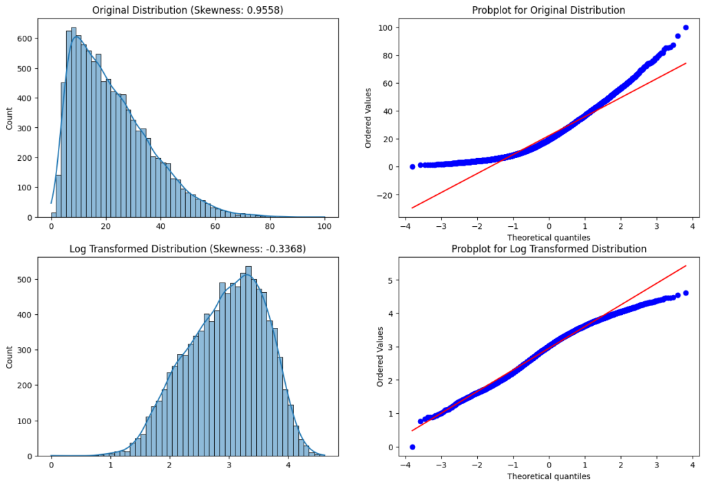
Log Transform Features that contain the value 0
The general problem with log transforming features that contain the value 0 is that the log of 0 is not defined (-inf).
Therefore you can use the little trick to add 1 to the value: log(x+1). Numpy has therefore a build-in function: np.log1p(x). In this case, the log1p transformation of the value 0 is still 0.
df['feature'] = np.log1p(df['feature'])Disadvantages of Log Transformation
- The main disadvantage of the log transformation is that it requires the input data to be positive.
Box-Cox Transformation
The Box-Cox transformation is a mathematical transformation that can be used to transform non-normal data into a more normal distribution. It was introduced by statisticians George Box and David Cox in 1964.
df['feature'] = scipy.stats.boxcox(df['feature'], lambda)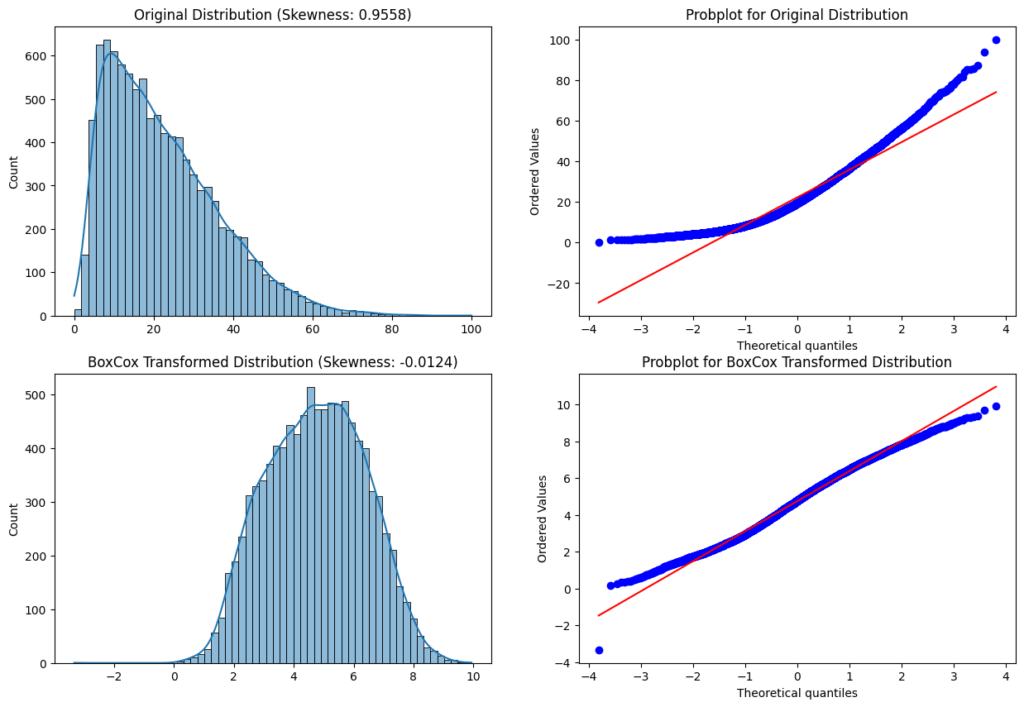
The value lambda is the power of the transformation. If you use the scipy library for the transformation you don’t have to set a value for lambda. If lambda is None a range of possible values is tested for maximizing the log-likelihood function.
w = \begin{cases} log(x) & \text{if } \lambda = 0, \\ \frac{(x-1)}{\lambda} & \text{otherwise} \end{cases}Notice that when lambda =1 the transformed data shifts down by 1 but the distribution does not change. In this case, the data is already normally distributed.
Advantages of Box-Cox Transformation
- The Box-Cox transformation has the advantage over other power transformations in that it can automatically determine the appropriate power to use based on the data.
Disadvantages of Box-Cox Transformation
- The Box-Cox transformation requires the input data to be positive, but the Yeo-Johnson transformation is quite similar and does not have the restriction that all values have to be positive.
Square Root Transformation
The square root transformation works analog to the log transformation by applying the square root to a variable or feature. When the square root transformation is applied to a positively skewed dataset, the transformed dataset will have a more normal distribution.
df['feature'] = np.sqrt(df['feature'])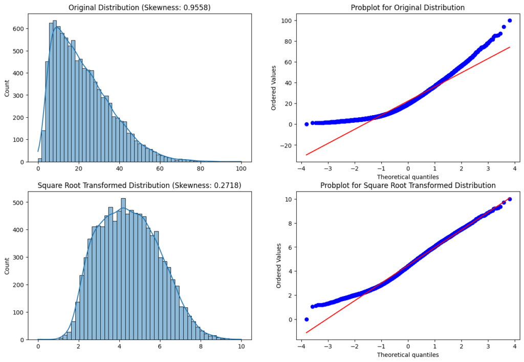
Advantages of Square Root Transformation
- The main advantage of square root transformation is, it can be applied to zero values.
Disadvantages of Square Root Transformation
- The transformation is weaker than the log transformation.
- The square root transformation can not be applied to negative values
Cube Root Transformation
The cube root transformation is a mathematical transformation that takes the cube root of a variable to make a distribution more normal. It is similar to other power transformations such as the square root and the logarithmic transformation but has different properties. The cube root transformation works by compressing large values and expanding small values.
df['feature'] = np.cbrt(df['feature'])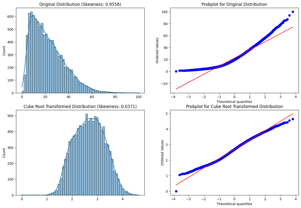
Advantages of Cube Root Transformation
- The main advantage of the cube root transformation is, it can be applied to zero and negative values.
Yeo-Johnson Transformation
The Yeo-Johnson transformation is a widely used data transformation technique that can be used to transform non-normal data into a more normal distribution. It was introduced by Robert Yeo and Robert Johnson in 2000 as an improvement over the Box-Cox transformation, which has limitations when dealing with data that contain negative values.
df['feature'] = scipy.stats.yeojohnson(df['feature'], lambda)The value lambda is the power of the transformation. If you use the scipy library for the transformation you don’t have to set a value for lambda. If lambda is None a range of possible values is tested for maximizing the log-likelihood function.
w = \begin{cases} \frac{((x+1)^\lambda -1}{\lambda} & \text{if } \lambda \neq 0, x>=0 \\ ln(x+1) & \text{if } \lambda =0, y>=0 \\ \frac{-((x+1)^{(2-\lambda)}-1)}{2-\lambda} & \text{if } \lambda \neq 2, y<0 \\ -ln(-x+1) & \text{if } \lambda =2, y<0 \end{cases}A value of lambda=1 produces the identity transformation.
Advantages of Yeo-Johnson Transformation
- The Yeo-Johnson transformation transforms zero, positive as well as negative values.
Inverse Transformation
The inverse transformation is very useful when the feature is a count or a rate, and we want to transform it into a continuous variable.
df['feature'] = 1/(df['feature'])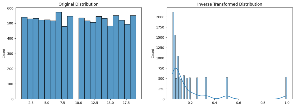
Advantages of Inverse Transformation
- The transformation can be used on a discrete variable or series.
Disadvantages of Inverse Transformation
The inverse transformation can only be applied to non-0 values.
Read my latest articles:
