In this article I show you how to create a basic classifier for the Kaggle Titanic competition. In the first part of this article we start with the simplest approach and build a solid foundation for more complex machine learning models that include cross validation to increase the generalization of our model. In the second step we add grid search to find the best combination of hyperparameter for our machine learning algorithm and therefore increase the accuracy of the cross validated classifier. In our last and final step we build a sklearn pipeline that executed different tasks before and during the training of the classifier and also increases the accuracy.
First Basic Model
Import all Libraries
Like in our last notebooks, the first step is to import all Python libraries that we use in the Jupyter notebook. As always, I recommend printing the version of the library in case you must debug you code.
For the basic models, we use the following libraries:
- os to use operating system dependent functions. In our notebook, we will check if a specific csv file exists. Os depends on your Python version and has no separate version.
- Pandas as always to handle our training and test dataset
- Numpy for some mathematical functions
- For visualizations I use seaborn in combination with matplotlib again
- For the machine learning part of the notebook, we use different functions of the sklearn library
To make the code cleaner, I turn off the warning of the Jupyter notebook.
# os: use operating system dependent functions
import os

# pandas: handle the datasets in the pandas dataframe for data processing and analysis
import pandas as pd
print("pandas version: {}". format(pd.__version__))

# numpy: support for large, multi-dimensional arrays and matrices and high-level mathematical functions
import numpy as np
print("numpy version: {}". format(np.__version__))

# sklearn: machine learning and data preperation
import sklearn
from sklearn.linear_model import LogisticRegression
from sklearn.metrics import precision_recall_curve, roc_curve, roc_auc_score, classification_report, confusion_matrix
from sklearn.preprocessing import StandardScaler
from sklearn.pipeline import Pipeline
from sklearn.compose import ColumnTransformer
from sklearn.model_selection import GridSearchCV
print("sklearn version: {}". format(sklearn.__version__))

# matplotlib: standard library to create visualizations
import matplotlib
import matplotlib.pyplot as plt
print("matplotlib version: {}". format(matplotlib.__version__))

# seaborn: advanced visualization library to create more advanced charts
import seaborn as sns
print("seaborn version: {}". format(sns.__version__))

# turn out warnings for better reading in the Jupyter notebbok
pd.options.mode.chained_assignment = None  # default='warn'


"""
pandas version: 1.3.1
numpy version: 1.20.3
sklearn version: 0.24.2
matplotlib version: 3.4.2
seaborn version: 0.11.1
"""
Load and Final Tune the Prepared Training and Test Data
In the last article we finalized the data cleaning and preparation. First, we load the training and test dataset that are saved as pickle file. I like to take a final view to all columns in the training data to check what features are the input for the machine learning algorithm and to make sure that the label has not been accidentally deleted during the preprocessing of the data.
# load prepared training and test dataset
df_train = pd.read_pickle('../03_dataCleaningPreparation/df_train_prepared_reduced.pkl')
df_test = pd.read_pickle('../03_dataCleaningPreparation/df_test_prepared_reduced.pkl')

# shjow all features that are used to train the algorithm
df_train.info()

"""
<class 'pandas.core.frame.DataFrame'>
RangeIndex: 891 entries, 0 to 890
Data columns (total 22 columns):
 #   Column        Non-Null Count  Dtype
---  ------        --------------  -----
 0   Pclass        891 non-null    float64
 1   SibSp         891 non-null    float64
 2   Parch         891 non-null    float64
 3   Family        891 non-null    float64
 4   TNlen         891 non-null    float64
 5   LeadingDigit  891 non-null    float64
 6   Fare_bin      891 non-null    float64
 7   Age_bin       891 non-null    float64
 8   x0_female     891 non-null    float64
 9   x1_C          891 non-null    float64
 10  x1_Q          891 non-null    float64
 11  x1_S          891 non-null    float64
 12  x2_adult      891 non-null    float64
 13  x2_children   891 non-null    float64
 14  x3_Alone      891 non-null    float64
 15  x3_Small      891 non-null    float64
 16  x5_Miss       891 non-null    float64
 17  x5_Mr         891 non-null    float64
 18  x5_Mrs        891 non-null    float64
 19  x6_NoPrefix   891 non-null    float64
 20  x6_pc         891 non-null    float64
 21  Survived      891 non-null    float64
dtypes: float64(22)
memory usage: 153.3 KB
"""
Before we can fit the data to the machine learning algorithm, we define the input and output of the training data:
- y-train is the output during the training of the classifier. In our case the label “Survived”
- x-train is the input during the training of the model and therefore, all features. When we first create y-train, then we can simply drop the label to create x-train.
- x-test is only a copy of the test dataframe.
# split the training and test dataset to the input features (x_train, x_test) and the survival class (y_train)
y_train = df_train['Survived']
x_train = df_train.drop(['Survived'], axis=1)
x_test = df_test
Create and Train the Logistic Regression Model
For our basic model, we use the logistic regression as classifier. First, we create a logistic regression object before we train the model by fitting the training data to the classifier.
# create an object for the logistic regression with default parameters
logreg = LogisticRegression()

# train the classification model
clf = logreg.fit(x_train, y_train)
So how well does our classifier predict if a passenger of the Titanic survived? The most used metric for classifications is the accuracy. Accuracy is defined as the ratio of all correctly labeled samples to the total number of samples. To get the accuracy of our model, we use the score function of our previously created logistic regression model. You see that with this simple machine learning model, we achieve an accuracy of 0.83.
# print the accuracy score for the training data
clf.score(x_train, y_train)

"""
0.8327721661054994
"""
But we can dive much deeper in the valuation of the classifier. But before we calculate additional metrics, we compute the predicted outcome of the training data “y_training_pred” and compute the confidence scores by using the decision_function for the training samples “y_scores”.
# predict the training outcome
y_training_pred = clf.predict(x_train).astype(int)

# predict probabilities
y_scores = clf.predict_proba(x_train)
# keep probabilities for the positive outcome only
y_scores = y_scores[:, 1]
Classification Report
Besides the accuracy, you should always look at the classification report. For the classification report I create a simple function that not only print the classification report to the Jupyter console, but also saves the classification report as a Python dictionary so that I am able to save some key metrics of the classifier as csv file.
To compute the classification report, we use the sklearn function with the true and predicted labels of the training data.
def plot_classification_report(y_train, y_training_pred):
    c_report = classification_report(y_train, y_training_pred, output_dict=True)
    print(classification_report(y_train, y_training_pred))
    return c_report

c_report_dict = plot_classification_report(y_train, y_training_pred)| precision | recall | f1-score | support | |
| 0 | 0.85 | 0.89 | 0.87 | 549 |
| 1 | 0.8 | 0.75 | 0.77 | 342 |
| accuracy | 0.83 | 891 | ||
| macro avg | 0.83 | 0.82 | 0.82 | 891 |
| weighted avg | 0.83 | 0.83 | 0.83 | 891 |
From the classification report, we get the following information separated by our two values 0 and 1 for the label “Survived”.
- The recall is the ability of a classification model to identify all relevant instances. Therefore, if we label all data as true, we get a recall of 1 but a worse precision.
- The precision is the ability of a classification model to return only relevant instances.
- The f1-score is the harmonic mean between precision and recall,
- The support is the number of samples of the given class in your dataset
In general, the metrics recall and precision interesting if your dataset is imbalanced, because for a highly imbalanced dataset a 99% accuracy is meaningless if only 1% of all passengers died when the Titanic sank.
In our case, you see that the logistic regression model is better at predicting the label 0 instead of 1, because the f1 score is higher.
In the second part of the classification report you see also the accuracy of 0.83 and some averages that are, in my opinion, not for interest in general.
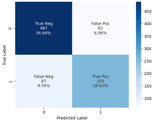
Confusion Matrix
One metric that is for interest if you have a binary classification problem, so only two different labels, is the confusion matrix. Each row of the matrix represents the instances in an actual class while each column represents the instances in a predicted class. Therefore, we can see how many labels are predicted right or wrong for each label.
To compute the Confusion Matrix we use the sklearn function.
def plot_conf_matrix(y_train, y_training_pred):
    group_names = ["True Neg", "False Pos", "False Neg", "True Pos"]
    group_counts = ["{0:0.0f}".format(value) for value in
                    confusion_matrix(y_train, y_training_pred).flatten()]
    group_percentages = ["{0:.2%}".format(value) for value in
                         confusion_matrix(y_train, y_training_pred).flatten()/np.sum(confusion_matrix(y_train, y_training_pred))]
    labels = [f"{v1}\n{v2}\n{v3}" for v1, v2, v3 in
              zip(group_names,group_counts,group_percentages)]
    labels = np.asarray(labels).reshape(2,2)
    sns.heatmap(confusion_matrix(y_train, y_training_pred), annot=labels, fmt="", cmap='Blues')
    plt.xlabel('Predicted Label')
    plt.ylabel('True Label')
    plt.show()

plot_conf_matrix(y_train, y_training_pred)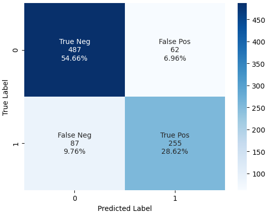
From the Confusion Matrix we see that
- 487 passengers that did not survived the titanic are predicted as dead -> True Negative (TN)
- But there are 87 passengers that survived the titanic that we also predicted as dead -> False Negative (FN)
- 255 passengers survived the titanic where the algorithms prediction is correct -> True Positive (TP)
- But there are 62 passengers that did not survive the titanic that we predicted as survived passengers -> False Positive (FP)
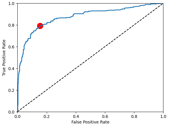
ROC Curve
The receiver operating characteristic (ROC) curve is another common tool used with binary classifiers and shows the true positive rate versus the false positive rate. From the curve you see that there is a tradeoff. The higher the TPR, the more false positives the classifier produces. The dotted line represents the ROC curve of a purely random classifier; a good classifier stays as far away from that line as possible (toward the top-left corner).
One way to compare classifiers is to measure the area under the curve, called AUC. A perfect classifier will have a ROC AUC equal to 1, whereas a purely random classifier will have a ROC AUC equal to 0.5. For our first basic model we achieved an AUC of 0.876.
To visualize the ROC curve, we use the sklearn function roc_curve and compute the area under the ROC curve with the roc_auc_score function. To visualize the optimal point of the ROC curve, we calculate the difference between the true and false positive rate. Now we use matplotlib to visualize the ROC curve as well as the dotted line for the random classifier and the point of optimum in red.
def plot_roc_curve(y_train, y_scores):
    fpr, tpr, thresholds = roc_curve(y_train, y_scores)

    roc_auc = round(roc_auc_score(y_train, y_scores), 3)
    print('Area Under ROC AUC: %.3f' % (roc_auc))

    optimal_idx = np.argmax(tpr - fpr)

    fig3, ax3 = plt.subplots()
    ax3.plot(fpr, tpr, linewidth=2)
    ax3.plot([0,1], [0,1], 'k--')
    ax3.axis([0,1,0,1])
    ax3.scatter(fpr[optimal_idx], tpr[optimal_idx], 200, marker='o', color='red', label='Best')
    ax3.set_xlabel('False Positive Rate')
    ax3.set_ylabel('True Positive Rate')
    plt.show()

    return roc_auc

roc_auc = plot_roc_curve(y_train, y_scores)

"""
Area Under ROC AUC: 0.876
"""
The ROC curve as well as the following evaluation metrics are more important for classifier where one class is more important than other classes. For example, if your job is to classify cancer patients it is more important to find all cancer patients even if that means flagging some patients as having cancer that actually do not have cancer. In this case you would increase the true positive rate even if you must disproportionately increase the false positive rate.
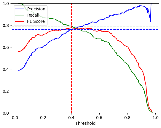
Precision-Recall-Curve
The Precision-Recall-Curve is another common tool used with binary classifiers. It is very similar to the ROC-curve, but instead of plotting the True Positive Rate versus False Positive Rate, the Precision-Recall-Curve plots the precision and the recall, where the true positive rate is another name for the recall, against the threshold.
The following function, called plot_precision_recall_vs_threshold created two different charts.
def plot_precision_recall_vs_threshold(y_train, y_scores):
precisions, recalls, thresholds = precision_recall_curve(y_train, y_scores)
# convert to f score
fscore = (2 * precisions * recalls) / (precisions + recalls)
# locate the index of the largest f score
ix = np.argmax(fscore)
print("Highest F1-Score: %.5f" % fscore[ix])
print("Threshold F1-Score: %.3f" % thresholds[ix])
print("Precision for Highest F1-Score: %.2f" % precisions[ix])
print("Recall for Highest F1-Score: %.2f" % recalls[ix])
fig1, ax1 = plt.subplots()
ax1.plot(thresholds, precisions[:-1], "b", label="Precision")
ax1.plot(thresholds, recalls[:-1], "g", label="Recall")
ax1.plot(thresholds, fscore[:-1], "r", label="F1 Score")
ax1.axvline(x=thresholds[ix], color='red', linestyle='--')
plt.axhline(y=precisions[ix], color='b', linestyle='--')
plt.axhline(y=recalls[ix], color='g', linestyle='--')
ax1.set_xlabel("Threshold")
ax1.legend(loc="upper left")
ax1.set_ylim([0,1])
plt.show()
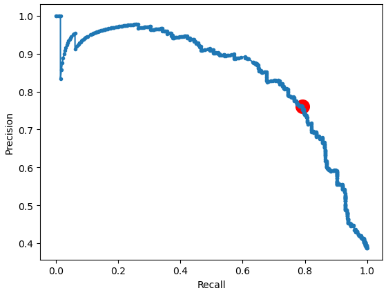
fig2, ax2 = plt.subplots()
ax2.plot(recalls, precisions, marker='.', label='Logistic')
ax2.scatter(recalls[ix], precisions[ix], 200, marker='o', color='red', label='Best')
ax2.set_xlabel('Recall')
ax2.set_ylabel('Precision')
plt.show()
plot_precision_recall_vs_threshold(y_train, y_scores)
"""
Highest F1-Score: 0.77650
Threshold F1-Score: 0.401
Precision for Highest F1-Score: 0.76
Recall for Highest F1-Score: 0.79
"""The first chart plots the precision, recall and F1 score against different thresholds and also shows the threshold of the highest F1 score. The second chart plots the precision against the recall and marks the combination of precision and recall for the highest F1 score.
Before we can create both charts, we use the sklearn precision_recall_curve function that computes all values of the precision, recall and thresholds. With the arrays of the precision and recall, we compute the F1 score and find the position in the array for the highest F1 score via the numpy argmax function.
With the position in the array, we can print the corresponding values of the highest F1 score, threshold and the corresponding precision and recall. Important to understand is that his F1 score, precision and recall are not the same as the F1 score in the classification report.
Classifiers perform differently for different threshold values because a classifier can only predict probabilities that are interpreted as crisp label class by comparing the probability with a threshold. Positive and negative predications can be changed by varying the threshold value.
In the following section I show you the differences in the F1 score and accuracy by varying the threshold, also called threshold moving. Therefore, I import the sklearn functions to compute the F1 score and the accuracy with the predicted labels and the real labels of the test set. First, we compute the f1 score and accuracy with the current predicted labels and the default threshold of 0.5. These metrics are also in the classification report.
Now we move the threshold where the F1 score is the highest. We have to re-compute the predicted labels by comparing the predicted probabilities with the threshold. The threshold for the highest F1 score was computed in the previous section and is 0.401. If the probability is equal or greater than the threshold, we classify the sample as 1 otherwise to 0. Now we also re-compute the F1 score and the accuracy and see that the F1 score is with 0.777 higher than 0.774 but we achieved a lower accuracy with 0.82, compared to 0.83.
from sklearn.metrics import f1_score
from sklearn.metrics import accuracy_score

print("Default Threshold (0.5)")
print("F1-Score: %.5f" % f1_score(y_train, y_training_pred))
print("Accuracy: %.5f" % accuracy_score(y_train, y_training_pred))
print("-"*50)

y_training_pred_f1 = (y_scores >= 0.401).astype('int')
print("Threshold Highest F1-Score")
print("F1-Score: %.5f" % f1_score(y_train, y_training_pred_f1))
print("Accuracy: %.5f" % accuracy_score(y_train, y_training_pred_f1))

"""
Default Threshold (0.5)
F1-Score: 0.77390
Accuracy: 0.83277
--------------------------------------------------
Threshold Highest F1-Score
F1-Score: 0.77650
Accuracy: 0.82492
"""
Optimize your classifier for different metrics
You see that depending on your metrics, you can optimize your classifier. For sklearn the threshold is optimized to achieve the highest accuracy, but if you want to optimize your threshold for another metric, you now know how to use threshold moving.
Create and Save Model Report
In later stages of the project, we will improve our first basic classifier and use different machine learning algorithms. Therefore, it would be very useful to save some model metrics in a csv file to compare different models.
I only want to use one csv file that does not exist. In later stages we want to read this csv file and add the metrics of the current classifier. For this reason, we first check if the csv exists. If so, we read the csv file as pandas dataframe. Otherwise, we create a new pandas dataframe with the following columns:
- Model is the name or identifier for the current classifier. For our first basic model, we use the name “fistBasicModel_LogisticRegression”.
- F1_0 is the F1 score for the label 0 that is saved in the classifier report.
- F1_1 is the F1 score for the label 1 that is also saved in the classifier report.
- Accuracy is the accuracy of the model with threshold 0.5.
- And the ROC_AUC score was the area under the ROC curve.
After we append the data of the current model, we save the pandas dataframe as csv file and print the current report that contains only one line from the current classifier.
# if there is already a saved classification report from previous models, read the classification report
if os.path.exists("classification_report.csv"):
    c_report = pd.read_csv("classification_report.csv")
# but if there is no saved classification report, create a new dataframe with the needed columns
else:
    c_report = pd.DataFrame(columns=['Model', 'F1_0', 'F1_1', 'Accuracy', 'ROC_AUC'])

# read the key data from the classification report to save the key data to a new dataframe
c_report_data = {
    'Model': ['firstBasicModel_LogisticRegression'],
    'F1_0':round(c_report_dict['0.0']['f1-score'], 2),
    'F1_1':round(c_report_dict['1.0']['f1-score'], 2),
    'Accuracy':round(c_report_dict['accuracy'], 2),
    'ROC_AUC': roc_auc
}

# append the key data from the classification report of the current model to the overall classification report
c_report = c_report.append(pd.DataFrame(c_report_data))

# save the classification report to the drive
c_report.to_csv("classification_report.csv", index=False)
Create Submission
Our first basic model is of course not the best model that we build and has therefore not the best results. But I want to build a function that creates the csv file for the submission on the Kaggle website. We can use the same function in every other Jupyter notebook when we want to submit our results. If we do not want to create the submission file, we can either delete the function or comment the line that executes the submission function.
The function is called create_submission and has the classifier itself and the features of the test set as parameter. First, we predict the test labels and then read the submission file that we downloaded from the Kaggle website in the raw data folder.
The submission file has a column “Survived” that we fill with our predicted test labels. The last step is to save the submission file as csv file.
def create_sumbission(clf, x_test):
    # predict the test values with the training classification model
    y_pred = clf.predict(x_test).astype(int)

    df_submission = pd.read_csv("../01_rawdata/gender_submission.csv")
    df_submission['Survived'] = y_pred
    df_submission.to_csv("submission_firstbasicModel.csv", index=False)

create_sumbission(clf, x_test)
Add Cross Validation to the Basic Model
In our basic model, we evaluated the model with the training data. The problem is that training and evaluating the model with the same dataset does not show how well the model performs on new data. If the model overfits or underfits the new data, the generalization is low, and the model is worthless.
Changes in Code
There are multiple methods to add cross validation but most of the times I used k-fold cross validation that involves splitting the training dataset into k folds. The first k-1 folds are used to train a model, and the holdout kth fold is used as the test set. This process is repeated and each of the folds is given an opportunity to be used as the holdout test set. A total of k models are fit and evaluated, and the performance of the model is calculated as the mean of these runs.
You can use your Jupyter notebook with the basic model and make the changes to add the cross validation.
In the first part of the notebook, we import two additional functions from the sklearn library: cross_val_predict and cross_val_score. In the third chapter of the notebook, where we train our model, we do not fit the training data to the logistic regression, but we use the cross_val_score function where the logistic regression function and the training data is an attribute. Also we set the number of cross validations to 10 and with n_jobs=-1 we use all cores of our PC for the training of the classifier.
scores = cross_val_score(logreg, x_train, y_train, cv=10, n_jobs=-1)
print("Accuracy: %0.3f (+/- %0.2f)" % (scores.mean(), scores.std() * 2))

"""
Accuracy: 0.828 (+/- 0.06)
"""
To predict the training labels, we use the second function that we imported, cross_val_predict. This function has the following arguments: the classifier, the training data, and the number of cross validations as well as the n_jobs. But the function has also the attribute method. To predict the training labels, we set the method to “predict” and with “predict_proba” this function outputs the probabilities.
# predict the training outcome
y_training_pred = cross_val_predict(logreg, x_train, y_train, cv=10, method="predict", n_jobs=-1).astype(int)

# predict probabilities
y_scores = cross_val_predict(logreg, x_train, y_train, cv=10, method="predict_proba", n_jobs=-1)
# keep probabilities for the positive outcome only
y_scores = y_scores[:, 1]
When you want to create the csv file for the submission, you have first to fit the model again, because during the cross validation we do not get any trained model back to use for the prediction of the test data.
def create_sumbission(clf, x_test):
    # predict the test values with the training classification model
    y_pred = clf.predict(x_test).astype(int)

    df_submission = pd.read_csv("../01_rawdata/gender_submission.csv")
    df_submission['Survived'] = y_pred
    df_submission.to_csv("submission_add_crossValidation.csv", index=False)

# train the classification model
clf = logreg.fit(x_train, y_train)

create_sumbission(clf, x_test)
All other parts of the code are the same and now we can compute all evaluation metrics and compare the results.
Compare the Results
When we compare the results of our first basic model and our current model with added cross-validation, we see that the accuracy stays at 0.83. In the confusion matrix, the true negative and false positive are also equal. Only 4 samples that were predicted correct with label 1 are now false. You can see the change from true positive to now false negative.

Therefore also our area under the ROC curve falls from 0.876 to 0.862.
If we take a look at the precision-recall-threshold-curve, we see that the F1 score is also lower compared to the first basic model. At a very high threshold you see that the precision drops very steeply. The same behavior is also seen in the precision-recall-curve. The precision can also drop to 0 and therefore computes an infinite F-score.
Highest F1-Score: 0.77650
Threshold F1-Score: 0.401
Precision for Highest F1-Score: 0.76
Recall for Highest F1-Score: 0.79
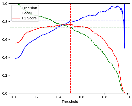
Highest F1-Score: 0.76758
Threshold F1-Score: 0.502
Precision for Highest F1-Score: 0.80
Recall for Highest F1-Score: 0.73
But why drops the precision at a high threshold? As the threshold increases, the model classifies fewer samples as positives. At a very high threshold, the model classifies no samples as positives and therefore the TP rate is 0 and with it also the precision (=TP/(TP+FP)) and the recall (=TP/(TP+FN)).
You also see that we could not compute the F-Score, because the multiplication of the precision and recall is the dominator when calculating the F-Score.
In total we increased the generalization by adding cross-validation to our model, but we do not increase the accuracy. Therefore we add grid search to our model with the objective to find the best parameter combination for our logistic regression model.
Add Cross Validated Grid Search to find the best Parameter
Changes in Code
To add grid search to the model, we add a parameter grid that is a python dictionary with the parameters that your machine learning model offers to change. On the sklearn website you find for every machine learning model the parameters with additional information.
In my case I try change the norm of the penalty, change the inverse regularization strength and the algorithm to solve the optimization problem. If you use grid search, every parameter combination is used to find the best accuracy. If you have a more complex machine learning algorithm and have a large parameter grid with many parameters and many values, it is recommended to use RandomizedSearch where you can define the total number of parameter combinations so that your model does not take hours to train.
# define the parameters for grid search
param_grid = [{
    'penalty': ['l1', 'l2', 'elasticnet'],
    'C': [0.01, 1, 2],
    'solver': ['newton-cg', 'lbfgs', 'liblinear', 'sag', 'saga']
}]
After adding the parameter grid, we create the Grid Search object that takes our logistic regression function as estimator and the parameter grid as attributes. Also, we define again the number of jobs to -1 and the number of cross validations to 10. With refit set to true (default option), after the best parameter combination is found, this combination is again fit to the training data. Therefore, we can directly use the predict and predict_proba function. Otherwise, you must select the best model from the grid search object with best_estimator.
With the verbose attribute, you can control how much information are displayed during the training process. I like to set verbose to 0 to get the fewest information.
# create grid seach object
grid_search = GridSearchCV(
    estimator = logreg,
    param_grid = param_grid,
    n_jobs = -1,
    refit = True,
    verbose = 0,
    cv=10)
During the training, we get some warning for infinite values that we do not have to consider.
We print the mean accuracy by using the best_score function of the grid search object and we can print the best parameter combination that was found.
# print the mean accuracy of the best grid combination and the configuration to the console
print('Mean Accuracy: %.3f' % grid_search.best_score_)

for key in grid_search.best_params_.keys():
    print(str(key) + ": " + str(grid_search.best_params_[key]))

"""
Mean Accuracy: 0.828
C: 1
penalty: l2
solver: lbfgs
"""
To compute the training outcome and the probabilities, we can use the same functions that we used in our first basic model, but our model is not the logistic model itself but the grid search object. Now we can run the evaluation functions and compare the results.
Compare the Results
For the Titanic dataset with our data preparation and the Logarithmic Regression function, adding the grid search improved our classifier only a bit. The precision for the negative label improved from 0.84 to 0.85 and the recall for the positive class improved from 0.73 to 0.75. The accuracy is equal with 0.828.
| precision | recall | f1-score | support | |
| 0 | 0.85 | 0.89 | 0.87 | 549 |
| 1 | 0.8 | 0.75 | 0.77 | 342 |
| accuracy | 0.83 | 891 | ||
| macro avg | 0.83 | 0.82 | 0.82 | 891 |
| weighted avg | 0.83 | 0.83 | 0.83 | 891 |
Comparing the confusion matrix, we see an improvement for the positive label. 4 samples that are a false negative without grid search are now a true positive after adding the grid search. Therefore, also the area under the ROC curve increases from 0.862 to 0.876.
But we can increase the model performance even further by adding a pipeline to our model. With a pipeline you can add multiple functions before training the dataset. The advantage is that the model stays lean, and the code is optimized in the background processes.
Build a Full Stack sklearn Pipeline
There are multiple steps that can be added via the sklearn pipeline. The most used or numeric data are feature transformations and dimension reduction.
Sklearn Pipeline without Dimension Reduction
In our current notebook, any feature reduction would not make sense, because we already use the reduced feature set from the data cleaning and preparation notebook. Therefore, we will only transform all numeric features with the standard scaler. For linear models like logistic regression, it is recommended to use the standard scaler over the min-max scaler, because after the standardization the mean of all features is 0 and the standard deviation 1. This form of normal distribution makes it easier to learn the weights that are initialized to 0 or a small random value close to 0.
Changes in Code
First, we add 3 additional functions in our section at the top, where we import the libraries. We import the pipeline function to be able to create a pipeline, add the function ColumnTransformer that enables us to apply different transformers to either all or only selected features and the last function that we must add is the transformer itself, in our case the standard scaler.
After we added the lines in the library section, we add a new section, where we create the pipeline. First, we define a variable transformer_num that contains the numeric features that are added to the standard scaler. In our case this are all columns of the training data. If we didn’t use the one-hot-encoding for the categoric features in the data preparation notebook, we could also define a transformer for the categoric features, where we apply the one-hot-encoding in the sklearn pipeline.
The second step is to create the column transformer that contains the different transformer. In our case we only have the transformer for the numeric feature, that we call “num”, use the standard scaler as transformer and apply the transformer to the columns that are saved in the variable transformer_num. With remainder set to “passthrough” we define that columns which are not transformed are passed through this pipeline step without any transformation. If you use the default setting for remainder, these columns are not passed through but deleted.
# numeric features that are Standard Scaled
transformer_num = x_train.columns

# creation of column transformer
# features that are not in the transformer_cat or transformer_num array are passed through this pipeline step and not deleted
col_transform = ColumnTransformer(
    transformers=[
        ('num', StandardScaler(), transformer_num)
    ], remainder='passthrough'
)
In our last step we create the actual pipeline with the following steps:
- The first step is to transform the features of the training data. We call this step of the pipeline “columnprep” and execute the column transformer function.
- In the second step of the pipeline, we train our logistic regression model and call this step “classification”.
We must give each step of the pipeline a name because if we define the parameter grid for grid search, we must define which parameter is used for which step in the pipeline.
# define pipeline
pipeline = Pipeline(steps=[
    ('columnprep', col_transform),
    ('classification', LogisticRegression())
])
This leads us to our next change in the notebook because we must change the name of the parameter for the grid search dictionary. Every parameter is named the following way when a pipeline is executed: First the name of the pipeline step, then 2 underscores and at last the name of the parameter. In our case, we only have parameters for the logistic regression function and therefore add “classification__” ahead of the actual parameter.
# define the parameters for grid search
param_grid = [{
    'classification__penalty': ['l1', 'l2', 'elasticnet'],
    'classification__C': [2**n for n in range(-5,10)],
    'classification__solver': ['newton-cg', 'lbfgs', 'liblinear', 'sag', 'saga']
}]
The last change that we make is that in the cross-validated grid search function, the estimator is no longer the logistic regression but the whole pipeline.
# create grid seach object that takes not the classifier as estimator, but the whole pipeline
grid_search = GridSearchCV(
    estimator = pipeline,
    param_grid = param_grid,
    n_jobs = -1,
    refit = True,
    verbose = 1,
    cv=10)
Compare the Results
Comparing the results of the pipeline where we use the standard scaler with grid search and without the pipeline, we see that the mean accuracy is equal 0.828 and that there are minor changes in the confusion matrix, where one negative sample is not a true negative but also one true positive before is now a false negative. Also, the area under the ROC curve is slightly lower.
In summary: In our case using the standard scaler for the logistic regression function has no influence on the results of the classification model.
Sklearn Pipeline with Dimension Reduction
During the data cleaning and preparation, we saved the training and test dataset after the one-hot-encoding of the categorical features but before we reduced the dimension. You find the video for the data cleaning and preparation in den description section.
The question that comes in my mind is: would the result differ if we would use all features after the one-hot-encoding? I think we should test this case. Therefore, we save our current notebook with a new name so that 95% of the notebook is already programmed.
Changes in Code
Because we must add the dimension reduction to the pipeline, we import the necessary function in the first section of the Jupyter notebook. For the dimension reduction, we use the principal component analysis (PCA) that projects our data to a lower dimensional space. In contrast to truncated singular value decomposition also called TruncatedSVD, PCA centers the input data through a mean subtraction before performing the dimension reduction.
In the code block that defines the pipeline, we add the principal component analysis between the column transformation and the logistic regression and call the step “reducedim”.
# define pipeline
pipeline = Pipeline(steps=[
    ('columnprep', col_transform),
    ('reducedim', PCA()),
    ('classification', LogisticRegression())
])
Because we do not know the number of components that leads us to the best result, we also add the number of components after the dimension reduction as parameter to the grid search. Because the parameter is used in the pipeline step “reducedim”, we must call the parameter “reducedim__n_components”. You could define an array with fixed number of components, but my suggestion is to use a function that creates the array depended on the total number of features. The advantage is that you can use this function in all projects and not only for the Titanic Kaggle competition.
# define the parameters for grid search
param_grid = [{
    'reducedim__n_components': [50, 80, 100, 120],
    'classification__penalty': ['l2'],
    'classification__C': [0.125, 0.15, 0.2, 0.25, 0.25, 0.5, 1, 2, 5],
    'classification__solver': ['newton-cg', 'liblinear']
}]
Compare the Results
When we compare the results of the sklearn pipeline with dimension reduction, with the previous results where we implemented only the the cross-validated grid search, we see from the classification report that we increased the accuracy from 0.83 to 0.89.
| precision | recall | f1-score | support | |
| 0 | 0.91 | 0.91 | 0.91 | 549 |
| 1 | 0.86 | 0.85 | 0.86 | 342 |
| accuracy | 0.89 | 891 | ||
| macro avg | 0.89 | 0.88 | 0.88 | 891 |
| weighted avg | 0.89 | 0.89 | 0.89 | 891 |
That the classifier with added full sklearn pipeline performed can also be seen in the confusion matrix.
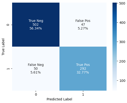
From the confusion matrix you see that we increased the true negatives from 487 samples to 502 and increased the true positives from 255 to 292 samples.
In summary you see that adding a sklearn pipeline that reduces the dimension of the dataset during the preprocessing of the classifier and adding a cross-validated grid search to find the best combination of parameters is a powerful tool to improve your machine learning algorithm.