When I start a new data analysis it helps me to have a fixed plan that I know how to execute. Therefore I do not get stuck by all the possibilities that a new dataset offers. In this article I show you my 3 steps that I do with every new dataset along with other helpful tips that improved my structure and productivity.
Find the Code on GitHub
You find the Jupyter notebook that I used in this article in my GitHub repository.
Because I do Kaggle competitions and the data analysis is the part before I do the data preprocessing and building the machine learning algorithm I will use the Kaggle Boston House Pricing dataset as example for this article.
General Tips for the Data Analysis
– Create a copy of your dataset so that your original dataset is save in case you overwrite the file
– I like to work in a Jupyter notebook, because I can make comments in markdown in the Jupyter notebook and see the output of every code block as well as all figures when I restart the notebook.
Load the dataset as Pandas DataFrame
My preferred tool to handle data in python is to use a pandas DataFrame. When you load your data, for example a csv file, to a pandas DataFrame, there are a lot of parameters that are very hand to use.
In the following example I wan to read the training csv file from the Kaggle Boston House Pricing. It is not wrong to read the whole csv file and using no attribute, but I want to show an example what these attributes can do.
import pandas as pd

df = pd.read_csv(
    filepath_or_buffer = 'train.csv',
    index_col = "Id",
    nrows = 200,
    converters = {
        "SalePrice": lambda x: float(x)*0.89 # converting the sales price from dollar to euro
    }
)

df.shape
"""
(200, 80)
"""

df.head(5).T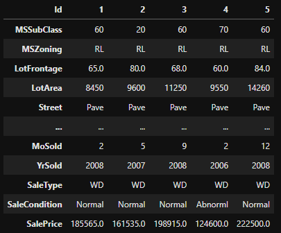
So lets get over the attributes that I used in this example while reading the csv to a pandas DataFrame:
- filepath_or_buffer: the path to your csv file (most of the time you only put the path inside the brackets without the attribute name
- index_col: the column in the table that should be used as index for the pandas DataFrame. If you do not have an index column, there is one created for you dataset
- nrows: is in my case very important because it limits the rows that are read in. In my case I limit the number of rows to 200. If you have a very large csv file with millions or billions of rows, it does not make any sense to read all samples while creating your data analysis. To reduce the time loading and computing the python script, use only a few samples to create your script. If your script is implemented you can increase the number of rows or read all rows to compute the final results for the data analysis.
- converters: is handy if you must convert units or currencies (for example dollar to euro). The attribute takes a dictionary where every column you want to convert is the key. With a lambda function you can define the computation that is done for every sample during the creation of the DataFrame. In my case I converted the sales price from dollar to euro and because the sales price is initially recognized as string, I use the float function to get the numeric data typ for the sales price. Otherwise I could not multiply a string by a numeric value.
You find all attributes in the pandas documentation.
Print the first few lines of the Dataset
After loading the dataset in a pandas DataFrame, I want to see the first lines of code to get a general understanding for the dataset. When you are working in a Jupyter Notebook you will have the problem, that not all columns are shown when you have not only a couple of columns. Therefore, you can set the option in pandas that all columns should be shown.
# settings to display all columns
pd.set_option("display.max_columns", None)

# show the first 5 columns
df.head(5)
When I am looking at the first few columns I am looking for the following points:
- can I already see NaN values?
- are there columns that I do not understand?
- are there columns with a value ranges that I did not expect?
Create a Statistic Report of the Dataset
From the first few lines of the dataset you can get a basic understanding, but it is more important to get some knowledge of the whole dataset. For this reason we create a statistic report for all numeric and categoric columns. For the visualization use the transpose function.
Use a statistic relevant number of samples
At the beginning of the script we limited the number of samples that we read to 200. Based on the total samples of your dataset, you have to decide what number of samples are fine for the statistic report. If you can read all samples for the static report, I would always read all samples. If you need all samples is also dependent on the structure of your dataset. For example if you have a time series from a machine it is more likely that you have missing values in batches and not distributed over the whole dataset.
df.describe().transpose() # for numerical features
df.describe(include="0").transpose() # for categorical features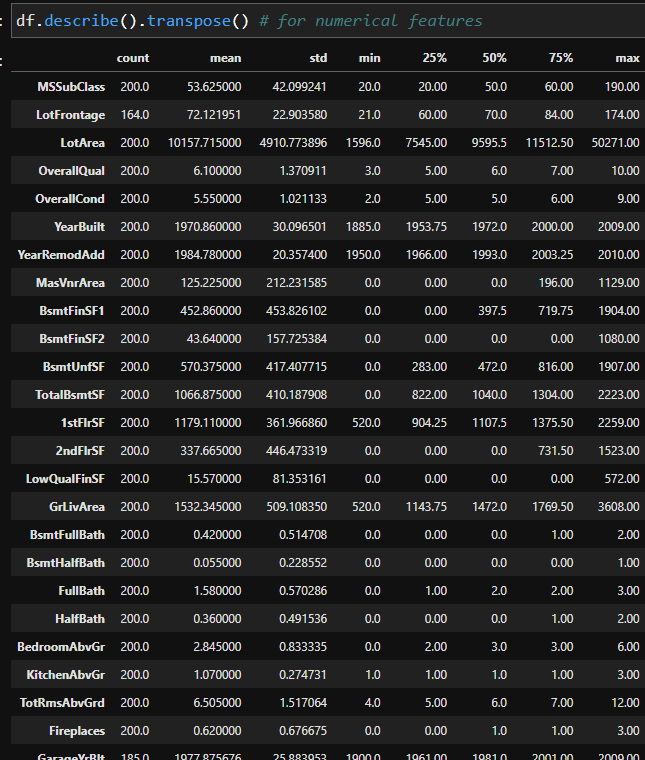
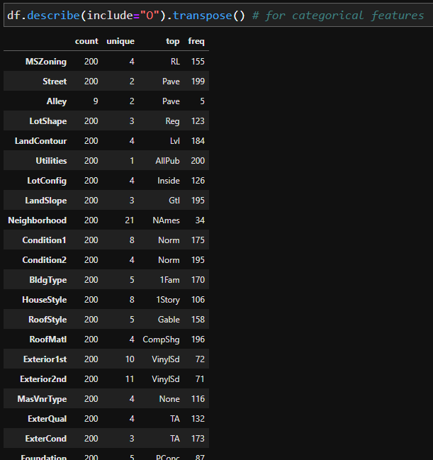
From the statistical report, you can get the following information
- How many samples contain each dataset and are there any missing values? Compare the count column for different features. For example the numeric feature LotFrontage and the categoric feature Alley have missing values.
- Numeric features
- What is the mean of the numeric values?
- How is the general distribution of the numeric features? Compare the 25%, 50% and 75% percentile.
- Do the min and max values make sense?
- Are there possible outliers? Compare the max values with the 75% percentile and the min value with the 25% percentile.
- Categorical features
- How many unique values are in each category?
Visualize the every Column of your Dataset
If you do not have a target variable
For most data analysis projects, you don’t want to test the impact of all the columns in your dataset on a particular column. Therefore we visualize only the single column that we are interested in. I like to create a loop to visualize every column of the dataset. For the implementation we have to separate the numeric and categoric columns.
Visualization of numeric features without a target variable
for col in list(df.describe()):
    sns.displot(data=df, x=col)
    plt.show()
For the numeric features I like to plot the distribution to get a feeling if there are some outliers or if the scale is maybe edge peaked due to data that is lumped together into a group labeled “greater than”.
Visualization of categoric features without a target variable
for col in list(df.describe(include="O")):
    sns.countplot(x=col, data=df)
    plt.show()
For categoric features I create the countplot to see the frequencies of each category in the dataset.
If you have a target variable
For all supervised machine learning tasks you have a target variable that can be an ongoing number (regression task) or a category (classification task). Therefore we have to distinguish our visualizations into 4 parts
- Visualize the influence of a numeric feature to a numeric target variable
- Visualize the influence of a numeric feature to a categoric target variable
- Visualize the influence of a categoric feature to a numeric target variable
- Visualize the influence of a categoric feature to a categoric target variable
Visualize the influence of a numeric feature to a numeric target variable
import scipy.stats as stats

for col in list(df.drop("SalePrice", axis=1).describe()):
    graph = sns.jointplot(data=df, x=col, y="SalePrice", kind="reg")
    df_ = df[[col, "SalePrice"]].dropna(axis='index')
    r, p = stats.pearsonr(df_[col], df_["SalePrice"])
    phantom, = graph.ax_joint.plot([], [], linestyle="", alpha=0)
    graph.ax_joint.legend([phantom],['r={:f}, p={:f}'.format(r,p)])
    plt.show()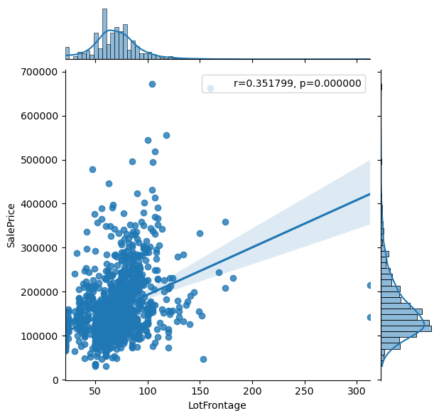
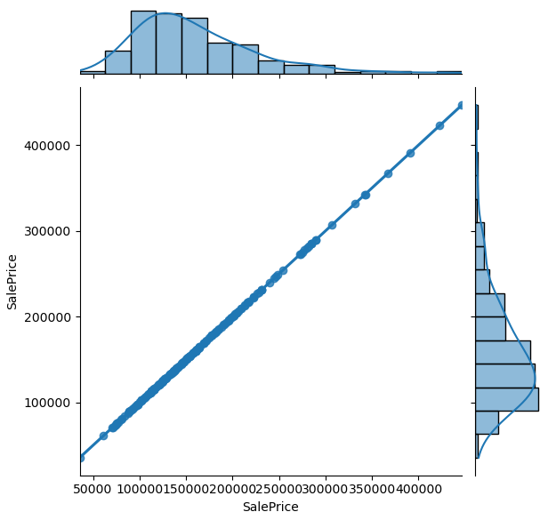
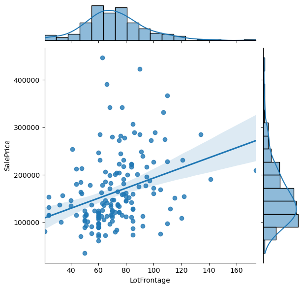
The jointplot combines the distribution and scatter plot and contains a lot of information. From the jointplot you also see a regression line with the Pearson correlation coefficient and the two-tailed p-value (for more information visit the Statistics for Data Science post). The objective is to get a feeling if there are columns in your dataset that explain the target variable as good as possible. Therefore you see that in the second plot, the target variable is plotted against itself and would perfectly explain the target variable.
Visualize the influence of a numeric feature to a categoric target variable
for colin list(df.describe()):
    sns.kdeplot(data=df_train, x=col, hue="Survived", common_norm=False)
    plt.show()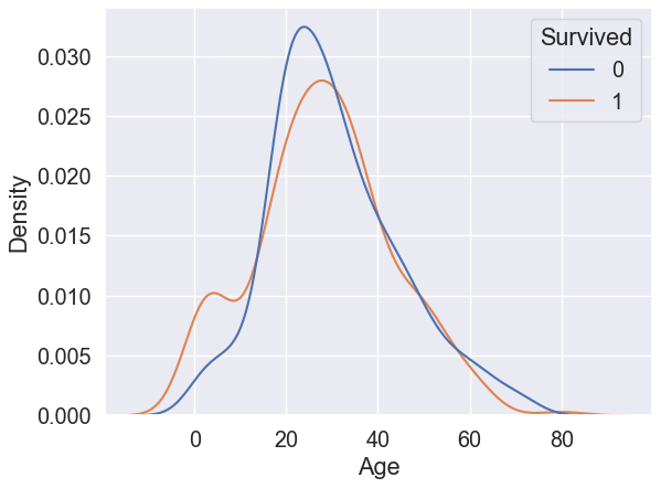
When we visualize the influence of a numeric feature on a categoric target variable, we use the kdeplot and get two different distributions in a binary classification task. Our objective is to find a feature in the dataset where the two distributions are best separated.
Visualize the influence of a categoric feature to a numeric target variable
for col in list(df.describe(include="O")):
    sns.catplot(x=col, y="SalePrice", data=df) # use kind="box" for many samples
    plt.show()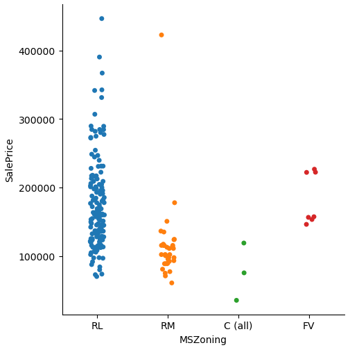
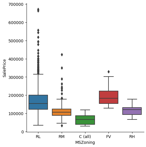
The influence of a category on a numeric variable is shown in the categorical plot. When we take a look at the categorical plot we wan to see classes that are not separated over the the whole range of the numeric variable. For only few samples you can use the scatterplot, but with increasing samples you should use the boxplot attribute.
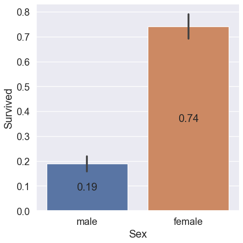
Visualize the influence of a categoric feature to a categoric target variable
for col in list(df.describe(include="O")):

    sns.catplot(x=col, y="Survived", data=df_train, kind="bar")
    plt.show()