Find Outlier by using the Residual Plot for Regression Problems

A more complex method to find outliers in regression models, compared to using the distribution of each feature, is to use the residual plots after you build and trained your regression model. The residual plot shows the error of the prediction. If the residual is a positive value (on the y-axis) the prediction was too low, and a negative value mean the prediction was too high. The objective is that all measurements are on a horizontal 0 line. From the following plot you can see if there are some value ranges that have a high error and could be declared as outlier.

Read the Boston House Price Dataset

The first part of the Jupyter notebook is to import all the libraries that we use in this article and also read the dataset that we use to find the outliers. As example dataset I use the Boston house prices dataset that you can find on the Kaggle website. Because outlier are only present in the numeric features of the dataset, we also create a list where all numeric features are stored in.

import pandas as pd
import numpy as np
import os
import seaborn as sns
import matplotlib.pyplot as plt

df = pd.read_csv(
    filepath_or_buffer = '../train_bostonhouseprices.csv',
    index_col = "Id"
)

# create a list of all numeric features
numeric_col = list(df.describe())

Prepare the Dataset for OLS Regression

To train our regression model we have to prepare our dataset. Normally you data preprocessing takes a couple more steps but I only focus on the following main preprocessing steps that I can train the OLS regression model:

• remove missing values
• rename column names that starts with a number in the name (only necessary for the OLS model of the statsmodel library)

import statsmodels.api as sm
from statsmodels.formula.api import ols

# drop all columns with a lot of missing values
df = df.drop(["Alley", "PoolQC", "Fence", "MiscFeature", "FireplaceQu"], axis='columns')
# drop all rows with missing values
df = df.dropna(axis='index')


# find all column names that start with a number and let them start with col_
for col in list(df):
    if col[0].isnumeric():
        df = df.rename(columns={col: "col_" + str(col)})

Train the Statsmodel OLS Regression Model

Because the input of the statsmodel is based on the programming language R, we can not simply define the pandas DataFrame as input. The columns must have the following schema as string:

1. dependent variable
2. separator “~”
3. all independent numeric features separated by a “+”
4. all independent categoric features separated by a “+” and in the following format “C(<categoric_feature>)

You will understand the schema from the program code 🙂

Because I do not want to write this schema by hand, I print all the numeric features separated by a “+” and all categoric features separated by a “+” and in the following format “C(<categoric_feature>) to the Jupyter output.

# print all numeric columns for the OLS model
col_numeric = list(df.drop("SalePrice", axis='columns').describe())
print(*col_numeric, sep = " +\n")

# print all categoric columns for the OLS model
col_category = list(df.describe(include="O"))
col_category = ["C(" + element for element in col_category]
col_category = [element + ")" for element in col_category]
print(*col_category, sep = " +\n")

The advantage is that I can now copy both strings to the program code to create the final string as input for the OLS model. The last step is to train the OLS regression model by fitting all attributes to the model.

# create the string for the OLS model
f = """
SalePrice ~
MSSubClass +
LotFrontage +
LotArea +
OverallQual +
OverallCond +
YearBuilt +
YearRemodAdd +
MasVnrArea +
BsmtFinSF1 +
BsmtFinSF2 +
BsmtUnfSF +
TotalBsmtSF +
col_1stFlrSF +
col_2ndFlrSF +
LowQualFinSF +
GrLivArea +
BsmtFullBath +
BsmtHalfBath +
FullBath +
HalfBath +
BedroomAbvGr +
KitchenAbvGr +
TotRmsAbvGrd +
Fireplaces +
GarageYrBlt +
GarageCars +
GarageArea +
WoodDeckSF +
OpenPorchSF +
EnclosedPorch +
col_3SsnPorch +
ScreenPorch +
PoolArea +
MiscVal +
MoSold +
YrSold +
C(MSZoning) +
C(Street) +
C(LotShape) +
C(LandContour) +
C(Utilities) +
C(LotConfig) +
C(LandSlope) +
C(Neighborhood) +
C(Condition1) +
C(Condition2) +
C(BldgType) +
C(HouseStyle) +
C(RoofStyle) +
C(RoofMatl) +
C(Exterior1st) +
C(Exterior2nd) +
C(MasVnrType) +
C(ExterQual) +
C(ExterCond) +
C(Foundation) +
C(BsmtQual) +
C(BsmtCond) +
C(BsmtExposure) +
C(BsmtFinType1) +
C(BsmtFinType2) +
C(Heating) +
C(HeatingQC) +
C(CentralAir) +
C(Electrical) +
C(KitchenQual) +
C(Functional) +
C(GarageType) +
C(GarageFinish) +
C(GarageQual) +
C(GarageCond) +
C(PavedDrive) +
C(SaleType) +
C(SaleCondition)
"""

model = ols(f, data=df).fit()

Evaluation of the OLS Regression Model (Creation of the Residual Plots)

After the OLS model is trained we can create a matrix of 4 charts for every input feature. One of the four charts is the residual plot that we can use to detect outliers. The following code shows how to save the 4 charts for every feature in a separate folder.

for col in col_numeric:
    fig, ax = plt.subplots(figsize=(15, 15))
    sm.graphics.plot_regress_exog(model, col, fig=fig)
    fig.savefig("regress_exog/{}.png".format(col))

The following residual plot shows the residuals from the feature “EnclosedPorch” as example.

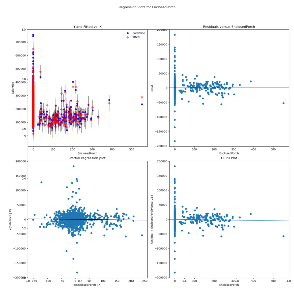
The residual plot shows the value of each sample on the x axis and the error of that sample on the y axis. We are looking for outliers on the x axis that have a significant distance to the horizontal line on the y axis. For the example feature ” EnclosedPorch” you see that there is one sample that has an error for a value higher than 500. From the plot you could therefore declare this sample as outlier and remove it from the dataset.

More information about this so called OLS Regression Plots can be could in the statistics for data science article.